1. The Problem of Evaluation

Evaluation is concerned with the determination of what the effects of a project or program are, and what is the relationship of the effects to specified variables, such as project inputs, client characteristics, or environmental characteristics.

At first glance, the problem of evaluating a project or program (henceforth we refer only to projects) may appear straightforward. The principles of statistical experimental design, as set forth by Sir Ronald A. Fisher in the 1920s, may be used to randomly assign "treatments" (program inputs) to "experimental units" (members of the target population), and the techniques of statistical analysis (e.g., the analysis of variance) may be used to determine an unbiased estimate of the treatment effects.

Through the 1930s, 1940s, and 1950s, statisticians, led by Dr. R. C. Bose, made great progress in the development of sophisticated experimental designs, such as balanced incomplete block (BIB) designs, partially balanced incomplete block (PBIB) designs, orthogonal Latin square designs, and fractional factorial designs. These designs could be used to simultaneously determine the effects of a large number of project variables on project effect, using only a modest number of experimental units (treated with particular combinations of levels of the treatment variables.

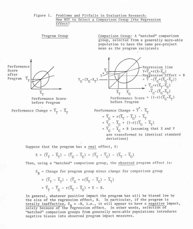
Despite the availability of the science of statistical experimental design, evaluation research has experienced a rocky road. Even when sound statistical experimental designs could have been applied to obtain unequivocal results, they often were not used. In many cases, simple after-the-fact "case studies" were applied to intuitively assess the project results. In other cases, comparison ("control") groups were formed by "matching" the comparison units to the treatment units on pre-measures of project outcome, or on various socioeconomic variables. While this procedure may appear reasonable (since it produces comparison groups that are similar to the treatment groups), it can produce disastrous results. It introduces what are known as "regression effects" -- biases in the estimated treatment effects caused by the (nonrandom) selection of units based on a variable that contains measurement error. (Note: in this discussion, we generally use the term "control group" to refer to a comparison group formed by randomized assignment, or to a naturally-assembled collection of experimental units (e.g., classroom, village) in the case in which the groups selected for treatment are randomly selected from the population of such groups; the term "comparison group" refers to a groups formed by any procedure -- e.g., randomized assignment, randomized selection of a pre-existing groups, or matching. This usage is not universal.)

Although the nature of regression effects has been known to statisticians since the time of Sir Francis Galton, behavioral scientists and economists have routinely ignored the problem, and often used this type of matching to construct comparison groups. This practice has resulted in a number of evaluation "disasters," such as the Westinghouse / Ohio University evaluation of the Head Start program. In this study, a comparison group was formed by matching -- identifying a group of individuals who were similar to the program clients based on a socioeconomic status score (an imperfect measure of the client's achievement ability). With this approach, the "controls" are usually selected from a generally more able population than the program recipients. Having been selected on the basis of an extreme score, in this case a low score, they will usually demonstrate a marked improvement upon retesting at the end of the program, simply because they were selected on the basis of an uncharacteristically low score at the beginning of the project. This artificial improvement is called a "regression effect," a "selection bias," or a "matching effect." In the Head Start evaluation, the study showed either no effects or harmful effects for the program -- a result almost surely due to regression effect biases caused by formation of the comparison group on the basis of matching on a variable imperfectly related to performance.

The advantage of using a statistical experimental design is that, if treatments (and non-treatment) are assigned randomly to experimental units, it is possible to obtain an unbiased estimate of program effect. Notwithstanding this tremendous benefit, however, there are many situations in which it is not practical or possible to assign treatments randomly. For example, in a study on smoking it is not possible to select a sample of human subjects and force some to smoke and some not to smoke (the assignment to the smoking and nonsmoking groups being made randomly). Or, in a social services program, federal law may prescribe who is eligible for benefits; benefits may not legally be withheld from randomly selected target populations for the purpose of conducting an evaluation.

In spite of numerous instances where political, ethical, or natural constraints have made it impossible to apply the randomization principle of experimental design, however, there are numerous instances in social and economic evaluation where randomization could have been applied to produce unequivocal evaluation results, and was not. There are two major reasons for this. First, the determination of what community receives an experimental program (e.g., a health or education program) may be political (e.g., the "worst" region gets the project). Second, the evaluation design effort may be initiated after the project has already begun, so that the evaluation researcher has no control over the treatment allocation. Since many project managers are not evaluation specialists, no attempt is made to formulate the project design to permit unbiased estimation of the project effects. The evaluation "design" must be formulated after the fact, given the treatment allocation.

2. Approaches to Evaluation

Because the use of statistical experimental design is not always present, alternative ways of conducting evaluations have been considered. In 1963, Donald T. Campbell and Julian C. Stanley published a monograph entitled, Experimental and Quasi-experimental Designs for Research, which described sixteen "quasi-experimental" designs for research. These designs attempted to reduce some of the threats to validity (biases) that result from the lack of randomized assignment of treatments (biases due to the effects of history, maturation of subjects, testing, instrumentation, regression, selection, and mortality). Some of these designs are based on "before-and-after" comparisons, whereas others are based on the use of a "comparison" group that is not formed by randomized assignment of individuals to the treatment and comparison groups.

Many years have passed since Campbell and Stanley introduced their work, and it is now considered that most of the quasi-experimental designs they discussed are poor alternatives to true experimental designs based on randomization, because of the prevalence and magnitude of the systematic threats to validity and the inability of statistical estimation to remove their effect.

The quasi-experimental designs that seem most immune from threats to validity (biases caused by a lack of randomization) are the interrupted-time-series design and the regression-discontinuity design. The reason why these designs are better is that theoretically, if a linear statistical model can be specified that describes treatment effect as a function of various explanatory variables in such a fashion that the model error terms are not correlated with the explanatory variable or with each other, and if there are no measurement errors in the explanatory variables, then the usual method of estimation (ordinary least squares) can be used to produce unbiased estimates of the model coefficients. (The model coefficients indicate the average change in treatment effect per unit change in the explanatory variable if the explanatory variables are uncorrelated.) The regression-discontinuity design and the interrupted time series design are examples of linear statistical models.

The regression-discontinuity design is simply a linear regression model that contains a number of explanatory variables, one or more of which are treatment variables. The rationale for use of this design is the fact that the explanatory variables (other than the treatment variables) will account for, or "explain," most of the difference between the treatment and comparison groups, and that the unexplained difference will be due to the treatments. While this assertion cannot be proved from the data, it is logically plausible if the analyst can reasonably argue that the explanatory variables probably do explain differences in the treatment and nontreatment populations. It is generally considered, however, that the "adjustment" that occurs to the effect estimate by accounting for the other variables is not sufficient, so that while the bias may be reduced, it is not eliminated.

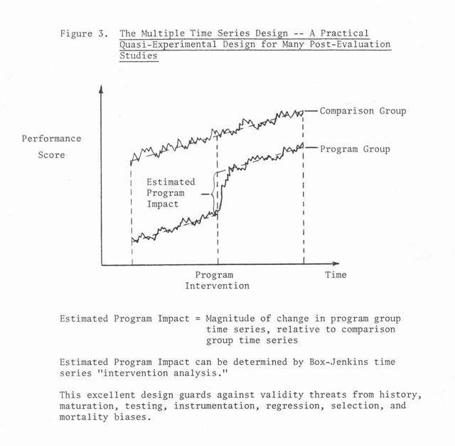
In the 1960s, Profs. George E. P. Box and Gwilym M. Jenkins introduced a family of time series models (autoregressive integrated moving average (ARIMA) models) that have gained wide acceptance in explaining time series phenomena. In 1970 they published a text entitled, Time Series Analysis, Forecasting and Control, and in 1975 Box and G. C. Tiao published a paper entitled, "Intervention Analysis with Applications to Economic and Environmental Applications." That paper shows how to use time series analysis to estimate the effect of program "interventions," or treatments, in situations in which the variable to be affected by the program is measured at frequent, regular intervals over time (e.g., unemployment). The procedure they describe is a generalized version of the interrupted-time-series design. It has gained wide acceptance as a means of estimating the effect of program interventions. Its validity rests on the same premise as the regression discontinuity design, i.e., that the other variables of the model (i.e., other than the treatment variables) explain all differences -- other than treatment -- between the treatment and nontreatment populations, the model error term is uncorrelated with the model explanatory variables (in particular, the treatment intervention) and each other, and measurement errors are not present in the explanatory variables. If a major, one-time change occurs in a nontreatment explanatory variable or in the model error term simultaneous with the introduction of the program intervention, the design cannot distinguish between the effect of that variable and the treatment variables. If the treatment variables are varied over time, however, this is unlikely to occur, and, if the model is properly specified, the estimation of the treatment effect coefficients will be unbiased.

In evaluating the effects of economic programs, econometricians often use linear statistical models ("econometric models") to represent the relationship of the program effects to various variables (program inputs, client characteristics, environmental variables, macroeconomic variables). (Many econometric models are "cross sectional" models, i.e., they do not include time series representations as do the Box-Jenkins or Kalman filter (state space) models.) This approach is an extension of the regression discontinuity design. As discussed above, this approach is valid if the model is properly specified (i.e., the model error terms are uncorrelated with the explanatory variables and each other, and there are no measurement errors in the explanatory variables). This condition cannot be empirically verified from the data, and the quality of the results depends in large measure on the model specification skill of the modeler, and the availability of data to measure the model variables.

While this approach has gained substantial support from economists over the past two decades, it has a serious shortcoming. The problem that arises is that regression models developed from passively observed data cannot be used to predict what changes will occur when forced changes are made in the explanatory variables, even if the model is well-specified. Such models measure only associations, not causal relationships. They describe only what will probably happen to the dependent variable (program effect) if the explanatory variables operate in the same way as they did in the past. If forced changes are made to the explanatory variables in a way that is different from in the past, there is no way of knowing whether they will produce the same results as were observed in the past. (This fact accounts for the fact that econometricians have been relatively unsuccessful in predicting the effect of changes in economic control variables on the economy -- the econometric models, although very elaborate (i.e., containing many variables and specification equations) were developed from passively-observed data (rather than from data in which forced changes were made to the explanatory variables).) The problem caused by incorporating passively-observed data into evaluation models is not as serious as for econometric forecasting models, because the program inputs are generally specified by the project planners (i.e., they are "forced", or "control," variables). Nevertheless, the evaluation project analyst must take special care in the interpretation of any model coefficients corresponding to variables whose values were not independently specified.

The most widely-used procedures for collecting data for evaluation include experimental designs, quasi-experimental designs, and sample survey. Issues dealing with the use of experimental and quasi-experimental designs were discussed above. With regard to the use of sample survey design, there are special problems that occur in the field of evaluation. The first problem is that the goal in some evaluation studies is to produce an analytical (e.g., regression) model that describes the relationship of program effects to various explanatory variables (program inputs, client characteristics, regional demographic and economic characteristics). The sample survey design that is needed to produce data suitable for the development of a regression model is called an "analytical" survey design. It is quite different from the usual sample survey design – a "descriptive" survey design, which is intended simply to describe the program effects in terms of major demographic or program-related variables. The approach to analytical survey design is quite different from that for descriptive survey design. In an analytical survey design, the objective is to develop a sample design that introduces substantial variation in the explanatory (independent) variables of the model. The objective in a descriptive survey design, on the other hand, is to develop a sample design that introduces substantial variation in the dependent variable (e.g., through stratification of the target population into internally-homogeneous categories, or "strata"). Standard sample survey design texts address the design of descriptive surveys, not analytical surveys.

The second important consideration in sample survey design for evaluation is the fact that use of the "finite population correction" (FPC) factor is generally not appropriate in evaluation applications. The FPC is a factor that reduces the variance of sample estimates in sampling without replacement from finite populations. Since the target populations for evaluation studies are finite, it might appear at first glance that this factor should be applied. It generally should not be applied, however, since the conceptual framework in an evaluation study is such that the goal is to make inferences about a process (i.e., the program), not a particular set of program recipients. This fact has been generally misunderstood in sample survey design for evaluation. The wrongful use of the FPC causes two problems. First, the estimated precision of the reported estimates may be grossly overstated. Second, the sample size estimates determined in the survey design phase to achieve desired precision levels may be grossly underestimated.

3. Vista's Approach to Evaluation

Vista's approach to evaluation depends on the timing of the evaluation effort and the resources that are available for evaluation. If the evaluation design is incorporated into the project design, it is possible to consider the full range of evaluation designs -- experimental designs, quasi-experimental designs, and analytic survey designs (including intervention analysis models and (cross-sectional) regression models). With heavy experience in statistical experimental design, time series analysis, and sample survey design, Vista can synthesize a number of alternative evaluation designs and work with the client to select one that is appropriate, given the available time, resources, and political constraints. Our expertise in the field of research design is very strong. Dr. Caldwell holds a Ph.D. in statistics, and specialized in experimental design in his Ph.D. program. He has developed new methodology for the design of "analytic" sample surveys to collect data for analytical evaluation models. He has over twenty years’ experience in evaluation, including the development of evaluation designs for development projects and the development of sample designs for nationwide and state evaluation studies in the US.

When the evaluation design can be done as part of the initial project design, the evaluation design can usually be much stronger than if the evaluation design is developed after initiation of the project (i.e., after the treatment allocation has been accomplished). The latter situation is very common, however, and Vista has developed an approach that addresses the evaluation problems inherent in it.

Given the often severe shortcomings of evaluation designs that are not based on a randomized assignment of treatments (program inputs), it is reasonable to ask what can be done if randomization is not possible or was not done. Such is often the case, since many evaluations begin after the project is well under way or even completed. The point is, however, that the use of the best quasi-experimental design or a cross-sectional regression model based on retrospectively-obtained data can be vastly superior to a poor alternative, such as an ex-post case study evaluation. Vista's approach to evaluation is to examine the evaluation situation, synthesize a number of reasonable alternative designs, and to select a "best" design, taking into account time, resource, and political constraints.

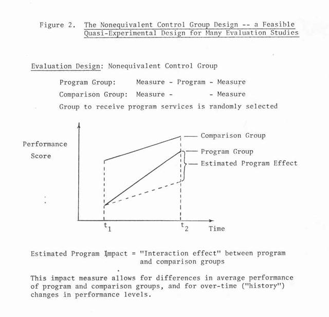
This approach has worked well. In the USAID-funded Economic and Social Impact Analysis / Women in Development project in the Philippines, Vista was responsible for identifying indicators, research designs, measurement instruments (data collections forms and questionnaires), and sampling plans for eighteen development project evaluations in the Philippines. Vista entered the project after all eighteen projects were under way, and so we had to accept the project treatment allocations as given. In spite of this constraint, we were able to make a very significant contribution to the improvement of the evaluation designs. Prior to our participation, many of the proposed designs were before-and-after case studies with no comparison groups (i.e., one-group pretest-posttest designs). After analyzing the situation and available resources, we proposed the use of the "nonequivalent control group" quasi-experimental design for several projects. This design utilizes "before-and-after" and control group data. The project effect is the "treatment x control group interaction," i.e., the difference in the change over time between the treatment and control groups. In this situation the control groups were randomly selected groups from the same population as the treatment groups, e.g., nontreatment villages in the same region as the treatment villages. A weakness in this design was that the groups selected for program treatment were not selected on the basis of randomization. Since the control groups were not formed by matching on a "pre-measure" of the program effect measure, the possibility of a "matching" bias in the impact estimates was minimized. Although the nonequivalent control group design may be subject to threats to validity, its use represented a significant improvement over the before-and-after case study (i.e., the one-group pretest-posttest designs), or "pre-experimental” designs, such as the one-shot case study or the static-group comparison design.

With regard to the choice of evaluation design, a principal factor to consider is whether the evaluation is to be essentially descriptive or analytical in nature. The descriptive approach simply addresses what happened (in terms of project results). The analytical approach attempts to determine the relationship of project outcome to various explanatory variables, including project control inputs as well as exogenous variables such as macroeconomic conditions, regional demographic characteristics, and client characteristics. Most evaluations are essentially descriptive in nature. They assess the project outcome, but provide only limited insight concerning the determinants of project outcome. The accomplishment of an analytical evaluation requires a substantially greater investment of resources, both for design (e.g., an analytical survey design vs. a descriptive design), data collection (i.e., collection of data on all of the explanatory variables of an analytical model), and analysis (e.g., regression analysis vs. crosstabulation analysis).

A key decision to be made in evaluation design concerns the choice of indicators, i.e., measures of project outcome. Ideally, what is wanted is a measure of effectiveness (MOE), which indicates what happened in terms of the ultimate goals of the project (e.g., employment, earnings, health, mortality). Often, however, it is not possible to measure the ultimate outcome (e.g., too many variables affecting employment may be operating concomitantly with the project variables to permit an unequivocal assessment of the effect of the project on unemployment). In this case, the evaluation centers on project outputs -- measures of performance (MOPs) -- which are logically linked to the ultimate effectiveness measure. For example, it may be possible to measure "number of meals delivered" to a target population, but not feasible to measure resultant decreases in mortality. In this case the linkage between improved nutrition and decreased mortality is accepted as a basis for using "number of meals delivered" as a measure of performance.

The preceding paragraphs have described some of the technical aspects of evaluation. In addition to the technical aspects, other aspects such as organizational and political aspects must also be considered. In the past, these other aspects were often ignored, leading to evaluation failures. To avoid this problem, Vista recommends that a procedure known as evaluability assessment be completed prior to each evaluation.

In the 1970s, it was realized that the investment in evaluation of government programs was not leading to more successful policies and programs, and a concerted effort was undertaken to determine why. Joseph S. Wholey and others working in the program evaluation group of The Urban Institute eventually identified a number of conditions which, if present, generally disabled attempts to evaluate performance. They developed the concept of "evaluability assessment" -- a descriptive and analytic process intended to produce a reasoned basis for proceeding with an evaluation of use to both management and policymakers. They developed a set of criteria which must be satisfied before proceeding to a full evaluation. This approach begins by obtaining management's description of the program. The description is then systematically analyzed to determine whether it meets the following requirements:

o it is complete

o it is acceptable to policymakers

o it is a valid representation of the program as it actually exists

o the expectations for the program are plausible

o the evidence required by management can be reliably produced

o the evidence required by management is feasible to collect; and

o management's intended use of the information can realistically be expected to affect performance

The object of an evaluability assessment is to arrive at a program description that is evaluable. If even one of the criteria is not met, the program is judged to be unevaluable, meaning that there is a high risk that management will not be able to demonstrate or achieve program success in terms acceptable to policymakers. The conduct of an evaluability assessment is considered to be a necessary prerequisite to evaluation.

In summary, then, Vista's approach to evaluation is to analyze the situation, to synthesize a number of alternative evaluation designs which are appropriate in view of time, resource, and political constraints, and, working with the client, to select the most appropriate design. In addition, prior to the evaluation, we recommend that an evaluability assessment be conducted. We are well-qualified to synthesize a suitable range of design alternatives, because of our qualifications and experience in statistical experimental design, sample survey design, and evaluation research.