Sample Survey Design for Evaluation (The Design of Analytical Surveys)
© 2009-2010 Joseph George Caldwell. All Rights Reserved.
Posted at Internet website http://www.foundationwebsite.org. 20 March 2009, updated 16 June 2010.
Contents
Sample Survey Design for Evaluation (The Design of Analytical Surveys) 1
1. The Design of Analytical Surveys. 2
3. Model-Dependent Approach. 7
5. Survey Design for Model-Based Applications. 17
6. Construction of Control (Comparison) Groups; Matching. 29
7. Sample Size Determination. 100
9. A Note on Random Numbers. 163
Appendix A. A Procedure for Designing Analytical Surveys. 164
Selected References in Sample Survey Design and Evaluation. 201
Note: This focuses on design of sample surveys for evaluation, not on analysis. Design and analysis go hand-in-hand: the design should be structured to enable and facilitate planned analysis, and the analysis must match the design (i.e., take into account the features of the design, including its structure and sampling methods). For this reason, this article includes some general consideration of analysis. Analysis of survey data will be addressed in a later article.
1. The Design of Analytical Surveys
Most sample surveys are conducted to make inferences about overall population characteristics, such as means (or proportions) or totals. The population under study is viewed as fixed and finite, and a probability sample is selected from that population. The statistical properties of the sample are defined by the sample design, the sample selection method and the population, not by any underlying properties of the process that created the population. These kinds of sample surveys are referred to as “descriptive” surveys.
In some instances, it is desired to make inferences about the process that generated the population, such as a test of the hypothesis about population characteristics (e.g., that two population subgroups (domains) could be considered to have been generated by the same probability distribution). In this case, the goal is to develop a mathematical model that is a reasonable description of the process that generated the population data, or that describes relationships among the variables that are observed on the population elements. The particular population at hand (the subject of the sample survey) is viewed as a sample from this process. Surveys conducted to assist the development of mathematical models are referred to as “analytical” surveys.
It does not make sense, in a descriptive survey, to test the hypothesis that two finite-population subgroups have different means. The means of any two population subgroups of a finite population are virtually always different. Tests of hypothesis about differences make sense only in the context of an analytical survey and conceptually infinite populations (such as the hypothetical outcomes of a process). (For the same reason, use of the “finite population correction” is not applicable to analytical surveys.) Similarly, it does not make sense to test the hypothesis that the mean of the population or a subpopulation equals a specific value – for descriptive surveys, it is estimates (point estimates and interval estimates) that are of interest, not tests of hypothesis. It is essential to decide on the conceptual framework for a survey (descriptive or analytical) prior to the design and analysis.
During the early period of the development of the theory of sample survey, up to about 1970, work in developing the theory of sample survey focused on the design of descriptive surveys. Standard textbooks on the subject, such as William G. Cochran’s Sampling Techniques (Wiley, 3rd edition, 1977) and Leslie Kish’s Survey Sampling (Wiley, 1965), describe methodology for designing and analyzing descriptive sample surveys. A popular elementary text on survey sampling is Elementary Survey Sampling 6th edition (Duxbury Press, 2005) by William Mendenhall, Lyman Ott and Richard L. Scheaffer. More detail on this topic are presented in the author’s previous note, Vista’s Approach to Sample Survey Design (1978), and in his course, Statistical Methods for Monitoring and Evaluation: A Comprehensive Survey Course. Course notes are posted at http://www.foundationwebsite.org .
The author specialized in the design of analytical surveys in his statistical consulting practice in the 1970s. At that time, there were no reference texts or articles on the subject. The methodology applied by the author to design analytical surveys was developed by drawing on his background in experimental design (in which he specialized in his PhD program as a student of Professor Raj Chandra Bose, the “father” of the mathematical theory of experimental design). During that time, he also promoted the use of experimental design to specify “run sets” for large-scale computer simulation programs. Since that time, a number of papers and books have been written on the topic of analytical survey design. These include “History and Development of the Theoretical Foundations of Survey Based Estimation and Analysis” by J. N. K. Rao and D. R. Bellhouse (Survey Methodology, June 1990);
Practical Methods for Design and Analysis of Complex Surveys 2nd edition by Risto Lehtonen and Erkki Pahkinen (Wiley, 2004); Sampling 2nd edition by Steven K. Thompson (Wiley, 2002); Sampling: Design and Analysis by Sharon L. Lohr (Duxbury Press, 1999); and The Jackknife and Bootstrap by Jun Shao and Dongsheng Tu (Springer, 1995).
The classification of surveys into two types – descriptive and analytical – was described in Cochran’s Sampling Techniques. The distinction between descriptive and analytical surveys is a little “fuzzy.” For example, a survey designed to describe the incomes of various population subgroups could be referred to as a descriptive survey, but if statistical tests of hypotheses about differences in income levels among the groups are to be made, the survey could be called an analytical survey. Rao and Bellhouse classify surveys and survey methodology into a slightly different and somewhat finer categorization: (1) design-based approach; (2) model-dependent approach; and (3) model-based approach or model-assisted approach. In the design-based approach, a probability sample is selected from the population under study (a fixed, finite population), and the nature of the sampling procedure suffices to define reasonable estimates of the population characteristics. How the population was generated is irrelevant – no probability (or other) model is defined to describe the generation of the population items. In the model-dependent approach, a purposive (non-probability) sample of observations is selected. Each observation is considered to be a realization (sample unit) from a specified probability distribution. The sample is usually assumed to be a sample of independent and identically distributed (iid) observations from the specified distribution, and (in any case) the nature of the joint probability distribution function of the sample determines what are good estimates for the quantities of interest, using standard sampling theory (e.g., as presented in Introduction to the Theory of Statistics, 3rd edition, by Alexander Mood, Franklin A. Graybill and Duane C. Boes (McGraw-Hill, 1950, 1963, 1974). In the model-based (or model-assisted) approach, a probability model is specified for the population units, and a probability sample is selected from the finite population under study. The sample is analyzed in a way such that the estimators are reasonable both for estimation of characteristics of the finite population under study and for estimation of the parameters of the assumed model and tests of hypothesis.
It could be argued that the model-dependent approach has nothing to do with “survey sampling,” which typically involves analysis of a probability sample from a fixed and finite population, and should not be considered as a separate category of survey sampling (leaving it to standard sampling theory and experimental design). Including it, however, facilitates discussion of the other two categories. The model-dependent approach is similar to experimental design, where a probability model is specified to describe the population items. For example, it is not the goal of an agricultural experiment or a clinical trial to describe the exact physical population that exists at the time of the survey, but instead to describe the properties of a hypothetically infinite population defined by a process of interest.
From a theoretical viewpoint, in the design of an analytical survey it is not necessary that all population items be subject to sampling, or even that the probabilities of selection be known. (It is required, however, that the probability of selection not be related to the model error term.) These conditions apply, however, only if the analytical model is correctly specified (identified, in the terminology of economics). A practical problem that arises is that this condition (of correct specification) can never be proved in practice, but only in simulation studies (where the model that generates the data is specified by the analyst). It is always possible that the model specification differs, in unknown ways, for different segments of the population (e.g., male / female, urban / rural, or different agricultural regions). The only sure defense against this possibility is to use probability sampling, where the probability of selection of all population elements is known and nonzero (it is not practical for all the probabilities to be equal in the design of analytical surveys). These probabilities may be set, however, in ways that enhance the precision of the sample estimates of interest (and power of tests of hypotheses of interest).
2. Design-Based Approach
The design-based approach is the standard approach to design and analysis of descriptive sample surveys. All of the older books on sample survey consider only this approach. As mentioned, the objective is estimation of means or totals for the population or subpopulations of interest. The major survey-design techniques for achieving high precision are stratification, cluster sampling, multistage sampling and sampling with varying probabilities of selection (e.g., selection of primary sampling units with probabilities proportional to size). Stratification may be used either to increase the precision of estimates of the overall population mean or total or to assure specified levels of precision of estimates for subpopulations of interest (called “domains of study”). Cluster and multistage sampling may be used for administrative convenience, to improve efficiency, or because sample units at different stages of sampling are of intrinsic interest (e.g., a survey that must produce estimates for schools and for students, or for hospitals and for patients). In cluster and multistage sampling, precision may be increased by setting the probabilities of selection of first-stage sample units proportional to unit size or a measure of size. Determination of number of strata and stratum boundaries may be done to improve precision of overall estimates or because certain strata are of particular interest.
The more information that is available about the population prior to conducting the survey, the better the job that can be done in survey design. In some instances it may be desirable to conduct a preliminary first-phase survey to collect data that may substantially improve the efficiency of the full-scale survey (double sampling, or two-phase sampling). In dealing with populations that are geographically distributed, it is usually the case that a simple random sample is not the best survey design, and large gains in precision or decreases in cost may be achieved through use of the survey-design methodologies mentioned.
A common problem in the design of descriptive sample surveys is that a number of estimates may be of interest, and the optimal design will vary for each of them. The survey designer’s goal is to determine a survey design that produces an adequate and efficient return of precision for all important survey estimates.
With respect to estimation of means (or totals) and standard errors, closed-form formulas are available for all standard descriptive-survey designs. It is possible to use simulation (resampling) methods to estimate sampling errors, but this is not necessary for standard descriptive-survey designs.
3. Model-Dependent Approach
In the model-dependent approach, the investigator has reason to believe that a particular probability distribution or stochastic model adequately describes the population, and taking this into account can improve the precision of estimates. The estimates may be estimates of population means or totals, but what is more likely are estimates of parameters of the probability distribution and estimates of differences (linear contrasts). In this approach, the population under study is viewed as having been generated by an underlying or hypothetical process. The population at hand is just one realization of a conceptually infinite set of alternative populations that might have been generated (in the “realization” of our world). In the model-dependent approach it is often the case that the investigator is interested in estimating relationships between variables, such as the relationship among several dependent variables observed on each sample unit, or on the relationship of a dependent variable to various independent (explanatory) variables.
In using the model-dependent approach, there is a basis for believing that the observations may be considered to be generated in accordance with an underlying statistical model, and it is the objective of the survey to identify (estimate) this model. This is a different conceptual framework for design-based surveys, where the objective is simply to describe the particular population at hand. This conceptual approach is the basis for experimental design. It is also the basis for statistical quality control and statistical process control, where the observations are produced by a manufacturing process. It is also the conceptual framework appropriate for evaluation research, where the outcomes of a program intervention are assumed to be produced by an underlying causal model. (For discussion of causal models, see Judea Pearl’s Causality: Models, Reasoning and Inference (Cambridge University Press, 2000).)
The model-dependent approach may be applied to both descriptive and analytical surveys. A few examples will illustrate this. In the first example, let us assume that we wish to estimate the mean and variance of the population income distribution, and that it is known (or reasonable to assume) that income follows a log-normal distribution (i.e., the logarithm of income is normally distributed). In the usual descriptive-survey approach, a probability sample may be selected, using one or more of the sample-design procedures identified earlier. For simplicity, let us assume that a simple random sample is selected (with replacement).
The standard approach in descriptive survey analysis is to make no assumptions about the probability distribution that describes the population elements, and to base the sample estimates (means and standard errors) on the sample design and the particular population at hand. The estimate follows from the design; how the population elements came about and the properties of any probability distribution that may be considered to have generated them is irrelevant. In the case of simple random sampling from a finite population, the sample mean is the estimate of the population mean, and the sample variance is the estimate of the population variance. The standard error (standard deviation) of the estimated mean is the square root of the ratio of the sample variance to the sample size.
In the model-dependent approach, however, we take advantage of the fact (assumption) that the underlying distribution of income is log-normal. We assume that the population represents a sample of independent observations from the same (lognormal) distribution, i.e., that the simple random sample of observations represents a sample of independent and identically distributed observations from this distribution.
Statistical theory tells us in this case that the best (minimum-variance, unbiased) estimates of the parameters of the lognormal distribution are obtained by estimating the mean and variance of the logarithms of the observed values. The estimates of the mean and variance of income are then obtained from these by appropriate transformations (i.e., the mean income is exp(mean + variance/2) and the variance of income is exp(2 mean + 2 variance) – exp(2 mean + variance), where “mean” and “variance” denote the mean and variance of the logarithm (which has the normal distribution).
The preceding is a very simple example of how information about an underlying probability distribution might be taken into account in determining population estimates. In most cases, the situation is more complex. What is usually the case is that the investigator wishes to estimate relationships among variables. In such cases, he is probably not interested in estimating overall characteristics (means or totals) of the population at hand. Interest focuses on the process (real or hypothetical) generating the observations, on relationships among variables, and on tests of hypothesis about the process that generated the particular finite population at hand. This underlying process may be described simply by a univariate probability distribution (e.g., the lognormal distribution in the example presented earlier), or a linear statistical model (e.g., multiple regression, experimental design), an econometric (structural equation) model, or a more complex model (e.g., a “latent variable” or path-analysis model).
In order to estimate the model parameters, the investigator typically engages in an iterative process of model specification, parameter estimation and model testing. If an estimated model does not pass the tests of model adequacy, the model is respecified and the process repeated until an adequate model is obtained. A key assumption in this approach is that the observed sample is an independent and identically distributed sample from the posited model, i.e., that the model is “correctly specified.” If this assumption holds true, good results will be obtained (for a sufficiently large sample). From a practical point of view, the problem is that the investigator usually does not know the correct model specification, and tries to determine it empirically from the data analysis. The difficulty that arises is that if the model is incorrectly specified, then the parameter estimates will be incorrect. This may or may not affect the quality of certain estimates derived from the model (e.g., least-squares forecasts corresponding to a model may be unbiased, even though estimates of the model parameters are biased).
In the model-dependent approach, it is not necessary to select a probability sample from the population (i.e., a sample in which every item in the population is selected with a known, nonzero probability (or the same unknown probability)). The investigator may select any sample he chooses, as long as he may reasonably assert that the sample is an independent and identically distributed sample from the posited distribution (or, if the sample items are not independent, he must specify the nature of the dependence). This precludes selecting a sample in a way that the likelihood of selection is related to the model error term (i.e., to the dependent variable). In the earlier example of the lognormal distribution of income, this is achieved by selecting a simple random sample from the population (i.e., a probability sample was in fact selected). In the case where a linear regression model describes the relationship of a dependent (response) variable to an independent (explanatory) variable, all that is required is that the model be correctly specified and that a reasonable amount of variation be present in the independent variable (and the colinearity among the explanatory variables be low) – any such sample from the population, whether a probability sample or not, will suffice.
As discussed above, the condition that the model be correctly specified is difficult or impossible to guarantee in practice. One of the usual conditions is that the model error terms be stochastically independent. This condition may be relaxed, as long as the nature of the dependence is taken into account. For geographically distributed populations, such as human populations, nearby (spatially proximate) population elements may be dependent (related). This fact should be taken into account when selecting the data sample (and analyzing the data). Observations taken over time may also be (temporally) correlated. The methods of time series analysis address means for modeling spatial and temporal correlations (e.g., time series analysis (Box-Jenkins models), geostatistics (kriging)).
The problem in designing the sample in the model-dependent approach is to have a good idea of what variables are important in the model, to assure a reasonable amount of variation in each of them, and to have low correlation among them. This is the same problem faced in experimental design. The branch of statistics known as experimental design describes good ways to select samples for the model-dependent approach. The only real difference between the design of model-dependent sample surveys and experimental design is that in experimental design the experimenter generally has considerable flexibility in setting the experimental conditions (values of the explanatory variables; for example, a research chemist may be able to set the time, temperature and duration of a chemical reaction at desired levels). The basic principles of experimental design are randomization, replication, local control and symmetry (these will be discussed further later). Whereas the field of experimental design includes elegant mathematical designs (e.g., fractional factorial designs, Greco-Latin squares, partially balanced incomplete block designs), the designs used in sample survey are generally very simple by comparison (e.g., cluster sampling, two-stage sampling, stratification, selection with variable probabilities, controlled selection).
The optimal sample design depends on what model is assumed. For example, if a zero-intercept regression model is assumed (yi = b xi + ei, where ei are a sequence of iid random variables of mean zero and constant variance), then the best sample to select is the n items in the population having the largest values of x, where n denotes the sample size. If in fact this model is incorrect, and the correct model involves an intercept (yi = a + b xi + ei) then the best sample is the one for which half the observations have the largest values of x and half have the smallest values of x. In this case, the previous sample (of the n items having the largest values of x) is a terrible sample design. If the model is not linear but curvilinear, then the second sample will be poor (we would want some observations in the middle of the range). As additional variables are added to the model, the difficulty of constructing a good sample design increases – this is the subject of the field of experimental design (e.g., fractional factorial designs; see, e.g., Experimental Designs, 2nd edition, by William G. Cochran and Gertrude M. Cox (Wiley, 1950, 1957)).
The important thing to realize with the model-dependent approach is that the optimal sample design, and good estimates, derive from the model assumed to generate the population units, not from the structure of the particular population (realization) at hand. In physical experiments, the experimenter generally has much control over the specification of combinations of experimental conditions, whereas in dealing with finite populations (such as program clients) this is often not the case (e.g., it may be impossible to orthogonalize the variables).
Reference texts dealing with estimation for the model-dependent approach include books on the general linear statistical model, such as C. R. Rao’s Linear Statistical Inference and Its Applications (Wiley, 1965); An Introduction to Generalized Linear Models 2nd edition by Annette J. Dobson (Chapman & Hall / CRC, 2002); An Introduction to Statistical Modeling by Annette J. Dobson (Chapman and Hall, 1983); Applied Regression Analysis by Norman Draper and Harry Smith (Wiley, 1966); and Applied Logistic Regression by David W. Hosmer and Stanley Lemeshow (Wiley, 1989).
4. Model-Based Approach
In the model-based (or model-assisted) approach, it is desired both to estimate overall population characteristics and to estimate parameters of the underlying probability model assumed to adequately describe the generation of that population (and to test hypotheses). In this case it is desired to select a probability sample from the population at hand, and to construct that sample such that it will produce good estimates of the population characteristics and the model parameters and tests of hypotheses. To accomplish the former, it is generally desired that the probabilities of selection be as uniform as possible. To accomplish the latter, it is desired that there be substantial variation in all dependent variables of interest, and that the correlation between independent variables that are causally (logically, intrinsically) unrelated to the dependent variable be low. For a probability sample from a finite population to produce (or even approximate) such a sample, the selection probabilities will usually vary considerably (often with some selection probabilities equal to one).
Books on sample survey design for descriptive surveys (design-based approach) describe a variety of different types of estimates. Two estimation procedures of descriptive-survey data analysis that may seem related to the model-based approach are ratio estimates and regression estimates. While both the design-based approach and the model-based approach may involve the specification and estimation of ratio and regression models, the ratio and regression estimates of descriptive survey data analysis have little to do with ratio and regression models of analytical survey data analysis. In descriptive survey data analysis, ratio and regression estimates are used to develop improved estimates of population means and totals, with little regard to any underlying probability model that may be considered to generate the population units. The ratio and regression estimates are simply numerical procedures used to produce improved estimates by taking into account ancillary data that may be correlated with the variable of interest. There is no consideration of an underlying model and whether it is correctly specified. The objective is to obtain good (accurate: high precision and low bias) estimates of population means and totals, not of parameters or properties of hypothetical models (such as regression coefficients or treatment effects) or tests of hypotheses (e.g., about a double-difference measure of program impact). (In particular, as mentioned earlier, it is not the objective in a descriptive survey to test hypotheses about equality of distributions or means of subpopulations, because for finite populations those distributions (or means) are (virtually) always different – there is nothing to test.) Furthermore, in ratio and regression estimation in descriptive-survey applications, the theory is developed for a single independent variable. In model-based applications, there are typically many independent variables (e.g., in a survey intended to develop an econometric model).
(Note that I do not use the terms outcome and impact interchangeably. The two are related, but not the same. The outcome of a job-skills program could be that the likelihood that a trainee gets a job is increased. If the number of jobs available is fixed, however, the total number of jobs remains unchanged, and the overall impact of the program is zero. The variables that affect impact may be quite different from those that affect outcome. For example, income or increase in income – outcomes – may be dependent on geographic location, but the double-difference measure of impact (interaction effect of program treatment and time) may not vary by geographic location at all.)
As mentioned, the “finite population correction” (FPC, the reduction in the variance for simple random sampling without replacement, owing to the fact that the population is finite) is not applicable to the estimation of underlying models (i.e., to analytical surveys). The inferences are being made about the process generating the finite population at hand, not about this particular realization of the process.
In the model-based approach, the role of a regression model is conceptually quite different from the role of a regression estimator in a descriptive (design-based) survey. In a descriptive survey, the regression estimate is nothing more than a computational mechanism for producing high-precision estimates. In the model-based approach, the objective is to determine a statistical model that is a valid representation of a process considered to have generated the population at hand. The validity (adequacy) of the model is assessed by conducting various tests of model adequacy, such as by examining the model error terms (“residuals”), and revising (respecifying and re-estimating) the model, if indicated. The book by Sharon L. Lohr, Sampling: Design and Analysis (Duxbury Press, 1999) discusses these concepts at a general level. For more on the topic of model adequacy, see any of the many books on statistical model-building, including books on econometrics and regression analysis. Examples include the books cited earlier (on regression analysis and the general linear statistical model) and: Mostly Harmless Econometrics: An Empiricist’s Companion by Joshua D. Angrist and Jörn-Steffen Pischke (Princeton University Press, 2009); Micro-Economics for Policy, Program, and Treatment Effects by Myoung-Jae Lee (Oxford University Press, 2005); Counterfactuals and Causal Inference: Methods and Principles for Social Research by Stephen L. Morgan and Christopher Winship (Cambridge University Press, 2007); Econometric Analysis of Cross Section and Panel Data by Jeffrey M. Wooldridge (The MIT Press, 2002); Matched Sampling for Causal Effects by Donald B. Rubin (Cambridge University Press, 2006); and Observational Studies 2nd edition by Paul R. Rosenbaum (Springer, 2002, 1995). These books relate to econometric modeling for evaluation. A comprehensive review of econometric literature is presented in “Recent Developments in the Econometrics of Program Evaluation” by Guido W. Imbens and Jeffrey M. Woodridge (Journal of Economic Literature 2009, Vol. 47, No.1, pp. 5-86). References on the general subject of econometrics (structural equation modeling) include: Econometrics 2nd edition by J. Johnston (McGraw Hill, 1963, 1972); Econometric Models, Techniques, and Applications by Michael D. Intrilligator (Prentice-Hall, 1978); Principles of Econometrics by Henri Theil (Wiley, 1971); Introduction to the Theory and Practice of Econometrics 2nd edition by George G. Judge, R. Carter Hill, William E. Griffiths, Helmut Lütkepohl, and Tsoung-Chou Lee (Wiley, 1982, 1988); and The Theory and Practice of Econometrics 2nd edition by George G. Judge, R. Carter Hill, William E. Griffiths, Helmut Lütkepohl, and Tsoung-Chou Lee (Wiley, 1980, 1985). (These are from my personal library, and many of them are old – there are many newer references available.)
5. Survey Design for Model-Based Applications
As described above, the problem in designing an analytical survey is to construct a survey design that has substantial variation in the independent variables of interest, low (or zero) correlation among causally (logically, intrinsically) unrelated independent variables. Also, all units of the population must be subject to sampling, and the probabilities of selection should be as uniform as possible, subject to achievement of the previous condition. (The probabilities of selection must be nonzero if it is desired to obtain unbiased estimates of population means or totals. Keeping the selection probabilities uniform generally increases the precision of these estimates (unless there is a good reason for varying them).)
There are several cases that may be considered, depending on the objectives of the investigation and the control that the survey designer has over selection of the sample units. In some applications, the goal is simply to develop a set of tables or a multiple regression model that describes the relationship of one or more dependent variables to a set of independent (explanatory) variables. An example of this would be the collection of survey data to develop an econometric or socioeconomic model of a population. In other applications, such as program evaluation (evaluation research, impact evaluation), it is of primary interest to estimate a particular quantity, such as a “double-difference measure” of program impact (in statistical terms, the interaction effect of program treatment and time), but because it is often not possible in socioeconomic evaluations to employ randomization to eliminate the influence of non-treatment variables on the impact measure, it is also desired that the survey enable the estimation of the relationship of program effects to other concomitant variables (ancillary variates, “covariates,” uncontrolled variables). (This is done for two reasons: because the relationship is of interest in its own right; and to adjust the double-difference estimate for differences among the four groups on which the design is based (treatment before, treatment after, control before and control after. The latter may be referred to a s model-based estimation of counterfactuals.) Finally, it may be possible to make use of the principles of experimental design to configure the design to reduce the bias or increase the precision of particular estimates, by means of techniques such as “blocking” or matching.
If it were not for the fact that we are sampling from a finite population (so that not all combinations of explanatory variables are possible), and for the desire to control the sample selection probabilities, the survey design problem (for a model-based application) would simply be an exercise in experimental design. The investigator would specify combinations of independent-variable values that corresponded to good variation in all explanatory (independent) variables and low correlation among them, and select units having these variable combinations from the population. This could be accomplished, for example, by employing an experimental design (e.g., a fractional factorial experimental design or a balanced incomplete block design), the Goodman-Kish method of “controlled selection,” or Cochran’s method of stratification on the margins. While these last two methods (of stratification) work well for small numbers of independent variables (such as two), they do not “scale” to situations involving large numbers of independent variables, as is common in the field of evaluation research. (The number of independent variables known in advance of the survey, and of interest in the data analysis, may be very large, including data from previous related surveys, from government statistical systems, or from geographic information systems. The number could easily be several hundred variables. The methods proposed by Kish and Cochran for multiple stratification are of no use in such a situation. They are appropriate for small numbers of design variables; they are intended simply to improve the precision of descriptive estimates, not to support the development of analytical models, which often include many variables.) When the number of independent variables is large, the number of combinations of stratification values (stratum cells) becomes very large, to the point where most stratum cells have zero or one population units and the number of cells containing one or more units exceeds the sample size (so that the standard theory for stratified sampling breaks down). Furthermore, a problem that arises in survey applications is that not every combination of variables exists (is possible or is represented in the population at hand), so that it may not be possible to accomplish orthogonality. Depending on how the selection is made, the probabilities of selection of the sample units may be poorly controlled, i.e., could be zero for some sample units and much more variable than desired or necessary for others.
Whereas in descriptive-survey design attention focuses on the dependent variables, in analytical-survey design attention focuses on the independent (explanatory) variables. In general, an analytical survey design will be very different from a descriptive survey design. This means that sampling plans for monitoring (i.e., descriptive surveys) are generally quite different from sampling plans for evaluation (i.e., analytical surveys).
The fact that the probabilities of selection usually vary widely for analytical survey designs (when they are known at all) has a strong effect on the estimation procedure. Since the sample weights (reciprocals of the selection probabilities) hence also vary widely, the weighted “regression estimates usually have low precision. For analytical surveys, it is generally preferable (when developing a regression model) not to use the weights (which is an option for a model-based or model-assisted approach, but not for the model-dependent approach). The estimates may be biased, but their precision will be high. If the model is correctly specified, this approach will not introduce bias, and if the model is reasonably valid, the mean-squared error of the estimates will be low.
There is another very significant difference between descriptive surveys and analytical surveys. Descriptive surveys tend to deal mainly with independent samples and minimizing correlations among sample units (to obtain high precision for estimates of totals and means), whereas analytical surveys tend to deal with correlated samples and deliberately introducing correlations into sample units (to obtain high precision for estimates of differences). Correlations certainly occur in descriptive surveys, such as in the case of cluster or multistage sampling (from intracluster / intraunit correlation), but it is generally sought to minimize these correlations. They usually decrease the precision of the estimates of interest (means and totals), and are introduced because they have substantial cost advantages (e.g., lowering of travel costs, administrative costs, or listing (sample-frame construction) costs). In analytical surveys, the introduction of correlations into the sample (in special ways) can increase the precision of estimates of interest (differences, regression coefficients). In such surveys, clusters (or first-stage sample units) are particularly useful in this regard, since information about them is often available prior to sampling, and may be used as a basis for matching or stratification (e.g., census enumeration areas, villages, districts).
The most important tool for increasing precision and reducing bias in analytical surveys is matching, and matching can be done only when some information is available on the sample units prior to conducting the survey. For ex-ante matching (i.e., matching before the sample is selected), some information is generally known about population aggregates (groups, clusters, areas), such as census enumeration areas or districts or regions, but it is typically not known about the ultimate sample units (e.g., households) – obtaining data on them is the primary purpose of doing the survey. For this reason, ex-ante matching can usually be done only on clusters, or “higher-level” sample units. Matching (pruning, matching, culling) may be done on the ultimate sample unit after the survey data are collected (ex-post matching). A descriptive survey uses clusters in sampling despite the intracluster correlation (because they enable cost savings which compensate for the associated precision loss); an analytical survey uses clusters because of it. Clusters enable matching, and are therefore the vehicle by which correlations are introduced into the sample.
Note that the intracluster correlation tends to decrease as the size of the cluster increases. For this reason, it is most desirable to match on the smallest units for which (pre-survey) data are available for matching. It follows that determination of sample size, which will be discussed in detail later, focuses on the lowest-level unit for which pre-survey data (suitable for effecting matching) are available. Descriptive surveys seek clusters with low intracluster correlations; analytical surveys seek clusters with high intracluster correlations (to increase the precision and decrease bias of comparisons, through matching).
During the 1970s, the author investigated alternative approaches to the design of analytical surveys. On the one hand, he investigated the use of formal optimization theory (Lagrangian optimization) to determine sample allocations that minimized the variance of estimates of interest. That approach proved to be unfruitful. The approach that proved most useful was a technique of setting the selection probabilities to effect an “expected marginal stratification.” With this approach, a design is iteratively constructed that satisfies a large number of expected stratification constraints, subject to keeping the probabilities of selection nonzero for all population items, and as uniform as possible. There are two major ways in which this algorithm is implemented, depending on whether it is desired to configure the design to maximize the precision of a particular treatment comparison (as is typically the goal of a program evaluation, such as estimation of a double difference): one way involves matching, and the other way does not. The method involves specifying the selection probabilities such that the expected numbers of units in each stratum cell are as desired. The method is general and can be applied in any situation. The method is used primarily to achieve a desired degree of spread in explanatory variables, but it can also be used to decrease the multicollinearity among them (by stratifying on interaction (or product) variables).
Appendix A describes the procedure in the case where it is desired to use the survey data to estimate a general linear model (e.g., analysis of variance, analysis of covariance, multiple linear regression), including the case in which it is desired to estimate a particular treatment comparison (e.g., a double-difference estimate of impact). It addresses the goal of the model-based approach of designing a survey that addresses both the estimation of model parameters and differences and tests of hypothesis (e.g., of a double-difference estimate of program impact) and estimation of overall population characteristics such as means and totals.
It is noted that, as in the case of design of descriptive surveys, the best design for (estimating or making tests of hypotheses about) a particular dependent variable will not be the best design for another dependent variable. For descriptive designs, this fact is accommodated by examining good designs for each of the important dependent variables, and selecting a design that is adequate for all of them. This is accomplished in the design of analytical surveys by including all independent variables for all models (i.e., associated with all dependent variables) in the algorithm simultaneously.
Note that the design should be matched to the analysis. This paper does not address analysis, except as it relates directly to design. Survey analysis is a major topic, and will be addressed in a later paper. If the design is not carefully considered, the analysis may be much more difficult, and its quality degraded. If the analysis does not take the design fully into account, much of the value of the design may be lost. It was reported recently, for example, that a high proportion of articles in medical journals analyzed data as matched (unpaired) samples, when they should have analyzed the data as matched pairs (“A critical appraisal of propensity-score matching in the medical literature between 1996 and 2003,” by Peter C. Austin, Statistics in Medicine, vol. 27: pp. 2037-2049, 2008).
Types of Evaluation Designs
Now that we have discussed some of the major aspects of sample design for analytical surveys, it is appropriate to summarize the three major types of analytical survey designs used in impact evaluation studies.
1. Experimental design. The distinguishing feature of an experiment (or “controlled” experiment) is that the experimenter controls the selection of experimental units and the assignment of treatment levels to them. The term “designed experiment” or “experimental design” implies that randomization has been used to select experimental units and to make the assignment of treatment levels to them. There are a great variety of experimental designs, but the most commonly used experimental design in evaluation research is perhaps the pretest-posttest-with-randomized-control-group design. Experimental design is the best approach to measuring causal effects, but it is often not feasible to allocate the treatment (program intervention) using randomization in socio-economic programs. If randomized assignment of the treatment is possible, then the influence of all other variables on outcome and the impact estimate is removed. Examples of experimental design are presented in William G. Cochran and Gertrude M. Cox’s Experimental Designs (2nd edition, Wiley, 1957). (Other related texts include George E. P. Box and Norman Draper’s Evolutionary Operation (Wiley, 1969) and Raymond H. Myers and Douglas C. Montgomery’s Response Surface Methodology (Wiley, 1995). E. S. Pearson and H. O. Hartley’s Biometrika Tables for Statisticians (Cambridge University Press, 2nd edition, 1958) contains tables of orthogonal polynomials.) An experimental design involves randomization at two levels – randomized selection of the experimental units, and randomized allocation of treatment levels to the selected units. A crucial assumption in experimental design is that the responses of the units are statistically independent (i.e., the error terms of the model are independent of the each other and of the explanatory variables). (An experiment is an investigation in which the assignment of treatments is controlled by the investigator. Studies in which the analyst uses passively observed data are referred to as “observational studies.”)
2. Structured observational (nonexperimental) study: Quasi-experimental design. If the data used for evaluation are not the result of a designed experiment, they are referred to as “nonexperimental data” or “observational data” or “passively observed data,” and the analysis of them is referred to as an observational study. An observational study may exhibit some of the structure of an experimental design, but randomization is not used, or used in a limited fashion, to select experimental units from a well defined population of interest and to assign treatment. When a considerable amount of structure is present, so that the observational study resembles a designed experiment in structure, it is usually called a “quasi-experimental” design. (For quasi-experimental designs, the term “comparison group” is often used instead of “control group” (although this usage convention is not universal). Experimental designs are sometimes referred to as “true” experimental designs, but this is redundant and misleading – all experimental designs involve randomized selection of experimental units from the target population and randomized assignment of treatment levels to them.) The most common example of a quasi-experimental design in evaluation research is the pretest-posttest design with a comparison (control) group selected by matching, or a “pretest-posttest-with-nonequivalent-control-group” design. The structure of a designed experiment is obtained by selecting the sample from the population according to the values of the design variables (such as treatment level), but the experimenter does not use randomization to determine the treatment variable levels. The control group is determined by matching, that is, by selecting comparison units that match the treatment units closely on a number of variables (that are known either prior to or after the survey). (To promote local control over time, the pretest and follow-up surveys may be implemented as panel surveys on the same units (e.g., households, businesses). Ideally, individual-unit matching is employed to construct the comparison group. With individual-unit matching, each treatment unit is matched to a similar non-treatment unit. (It differs from group matching, in which the treatment and comparison groups have the same distributions on match variables, but individual units are not matched.) Individual-unit matching ensures that the joint probability distribution of the treatment units and the non-treatment units are similar (so that selection biases are reduced), and also allows the use of a “matched-pairs” estimate of impact (via the double-difference estimate) (so that precision is increased). (In this article, attention has focused on the pretest/posttest/comparison-group quasi-experimental design. There are many other kinds of quasi-experimental designs. See Experimental and Quasi-Experimental Designs for Research by Donald T. Campbell and Julian C. Stanley (McGraw Hill, 1963, 1966), or Quasi-Experimentation: Design and Analysis Issues for Field Settings by Thomas D. Cook and Donald T. Campbell (Houghton Mifflin, 1979) for examples.) See Paul R. Rosenbaum’s Observational Studies 2nd edition (Springer, 2002, 1995) for discussion of observational studies.
3. Unstructured observational (nonexperimental) study: Analytical model. If there is no experiment (selection of experimental units or determination of treatment levels by an experimenter) and no useful structure, such as in a quasi-experimental design, then the situation is referred to as unstructured observational study, or an analytical model, or exploratory data analysis, or data mining. (The use of the term “analytical model” is a little misleading, since both the experimental design and the structured observational study (quasi-experimental design) involve the use of mathematical models to describe the process generating the data. It is used for lack of a better term.) For example, there may be no control groups at all, even formed by matching. A mathematical model (e.g., a general linear statistical model (such as a multiple regression model) or a nonlinear model such as a set of tables of means or a classification tree) is specified that describes the relationship of program outcome to a variety of explanatory variables related to program intervention, but there is not a well defined comparison group. This type of design is appropriate, for example, in the evaluation of road-improvement projects, where roads are typically selected for improvement for political or economic reasons, and program impact can be viewed as a continuous function of travel time or travel cost (which can be measured directly, reported by survey respondents, or estimated by a geographic information system). For example, a “path-analysis” (hidden variable) model may be used to describe the relationship of income to travel cost, and an engineering model may be used to describe the relationship of travel cost to road characteristics (which are affected by the program intervention). The ease with which an analytical model may be specified varies. For a road-improvement program, it may be generally agreed that the preceding model is a reasonable representation of reality. For a training program, it may be much more difficult to specify a reasonable model (so that use of a randomized experimental design is much preferred, and it is not necessary to worry about the relationship of impact to omitted variables). Note that the analytical model does not have to be linear, or even parametric. It may be specified, for example, as LOESS / LOWESS (locally weighted scatterplot smoothing) curves, bivariate (or more complicated) tables of means, or a classification-tree diagram of means (such as is produced by SPSS CHAID (Chi-square Automatic Interaction Detection) or Salford Systems CART (Classification and Regression Technique)). For complex relationships involving many variables, multiple regression models are commonly used. It should be recognized, however, that while the “fine tuning” or optimization models of industrial research are often linear, the “exploratory” models of evaluation research are often highly nonlinear. References on the general linear model include Norman Draper and Harry Smith’s Applied Regression Analysis (Wiley, 1966); David W. Hosmer and Stanley Lemeshow’s Applied Logistic Regression (Wiley, 1989); and C. Radhakrishna Rao’s Linear Statistical Inference and Its Applications (Wiley, 1965) (the last book is theoretical).
The methodology described in this article (and, in particular, in Appendix A) assists the development of analytical survey designs for cases 1-3 above.
Attribution of causality via open-ended questions. It may be that no experimental or quasi-experimental design is feasible, and it is not clear how to specify an analytical model describing the relationship of program outcome to program intervention (or no data relating to the explanatory variables of such a model are available prior to the survey). In this case, it may be that the best that may be done is to directly ask the respondents what they attribute observed changes (in impact variables) to. This is similar to the “focus-group” approach. (Including open-ended questions about the reasons underlying observed changes is also useful in the two preceding design types, since once we depart from a true experimental design with randomized control groups, there is always a question about the cause underlying observed changes.) For this type of study, the analytical-survey design methodology described in this article is not helpful, since it is not clear what variables should be used for an analytical model (or data on them is not available). In this case, the survey design will be similar to a descriptive-survey design (e.g. a simple random sample, stratified sample, or multistage design). The design may be stratified into domains for which it is suspected that the model specification may differ, but that is probably all that is done with respect to tailoring the design to assist identification of an underlying analytical model. This approach is really too “weak” (vulnerable to threats to (internal) validity) to be considered for a formal “impact evaluation,” but it may be useful as part of a monitoring system that may suggest hypotheses to test in a future rigorous impact evaluation and collect data useful for its design.
It is important to recognize that randomization (random selection of units and random assignment of treatment values to units) is not sufficient to guarantee good results, and elimination of all bias. The essential ingredient of a designed experiment (randomized trial) is that treatment assignment and response are stochastically independent. Randomized selection and randomized assignment of treatment values do not assure independence of response. A simple example serves to illustrate this. Suppose that we wish to evaluate a worker-development (training) program, which teaches basic job skills to workers, such as proper dressing, proper speech, résumé preparation, interview skills, dependability, and the like. The objective of the program is to increase employment and job retention. Let us suppose that the program is in fact very effective in increasing the likelihood that a person lands and keeps a job. Suppose however, that the number of jobs in the program area is fixed. If the graduates of the program get jobs and keep them, they are simply taking these jobs away from others. In this situation, even the use of a before / after / randomized-control-group experimental design would show that the program was very effective helping workers to get and keep and in increasing employment. The training program is effective only in redistributing existing jobs, however, not in creating new ones. The problem is that there is an interaction among the experimental units (individuals receiving training) – if one person gets a job, someone else has to lose one. This effect has been called the “Stable-Unit-Treatment-Value-Assumption” (or “SUTVA”). It is also called the “partial equilibrium assumption” or the “no-macro-effect” assumption. (For discussion, see Rubin, Donald B., “Bayesian Inference for Causal Effects: The Role of Randomization,” Annals of Statistics, vol. 6, no. 1, pp. 34-58 (1978); or Imbens, Guido W. and Jeffrey M. Wooldridge, “Recent Developments in the Econometrics of Program Evaluation,” Journal of Economic Literature, vol. 47, no. 1, pp 5-86, (2009); or Morgan, Stephen L. and Christopher Winship, Counterfactuals and Causal Inference, Cambridge University Press, 2007). Other examples of this effect are easy to cite. For example, a farmer-development program might teach farmers how to grow tomatoes more productively (efficiently), but if the demand for tomatoes is fixed, the increased production may serve simply to drive prices and farmer income down.
6. Construction of Control (Comparison) Groups; Matching
The Purpose and Nature of Matching
As mentioned, a useful experimental design in evaluation research is a “pretest / posttest / (randomized) control group” design. In this design, the program treatment is applied to a random sample of population units, and a similarly sized set of population units are selected as “controls.” A “baseline” survey is conducted to measure outcomes of interest prior to the program intervention, and a follow-up (“endline”) survey is conducted at a later time to measure outcomes after the program intervention. To increase “local control” (reduce experimental error) and thereby increase the precision of estimates and the power of tests of hypotheses, individual control units are usually matched to treatment. Also, a “panel” survey (longitudinal survey) is usually attempted, in which the same units are measured before and after the program intervention. The measure of program impact is the difference, between the treatment and control units, of the difference in outcome before and after the program intervention. In statistical terminology, this effect is called the interaction effect of treatment and time. In evaluation research it is referred to as a “double difference” or a “difference-in-difference” estimate (or measure). Because randomization is used to determine which units receive the program treatment, the influence (effect) of all variables other than the treatment variable(s) are removed from the estimate (i.e., the effect is averaged over these variables, as they are represented in the population from which sampling is done).
The purpose of forming similar groups or similar pairs of experimental units – one treatment and one comparison – is called “matching.” While matching is very useful for increasing the precision of estimates derived from an experimental design, it is even more useful in working with quasi-experimental designs. For quasi-experimental designs, matching is used both to increase precision and to decrease bias associated with lack of randomization in the treatment selection.
Matching is often referred to as “statistical” matching, for a number of reasons. First, the criteria for assessing the need for matching and the quality of a match are statistical in nature, dealing with concepts such as precision, bias, accuracy, probability, probability distributions, conditional distributions, conditional expectations and conditional independence. Second, statistical models, such as logistic regression models, are often used as part of the matching process. Third, generalized distance measures such as are used in statistics (e.g., Mahalanobis distance) may be used during the matching process.
A problem that arises in evaluation of social and economic programs is that it is often not feasible to randomize the assignment of the program treatment to population units (i.e., it is not feasible to use a (randomized) experimental design, and a quasi-experimental design is used instead). This problem arises for many reasons, including the fact that all members of the population may be eligible for a program, or the program may be offered on a voluntary basis and not all members of the population choose to apply. In this case, biases may be introduced into estimation of impact, because the treatment group and the comparison group may differ substantially with respect to one or more variables that may affect outcome. In an attempt to reduce selection bias, what is usually done is to form a comparison group by selecting a sample of population units that are similar to the treated units in variables (known prior to the survey) that may have an effect on program outcome or may have affected the likelihood of selection into the program. The treatment and comparison groups are made similar through the process of matching.
In an experimental design, matched pairs of experimental units are formed and one of them is randomly assigned to treatment. In a quasi-experimental design, the treatment units have already been selected. If the population of treatment units is small, all of them may be used for the evaluation study. If the population of treatment units is large, a sample may be selected from it (according to an appropriate sample design). In either case, for a quasi-experimental design the matching of comparison units is done after selection for treatment. The process of selection of the comparison-group items is done in a way such that the empirical probability distribution of the match variables is as similar as possible for the treatment and comparison groups. To increase the precision of the estimate, it is generally desirable to match each (individual) treatment unit to a similar comparison unit, (i.e., to use matched pairs as a means of promoting local control), not simply to match the groups overall (i.e., to cause the distribution of the match variables to be the same). For matching of individual units to be effective in increasing precision, the pairs must be matched on variables that are related to outcome (not just to selection for treatment).
The objective of matching may be to match individual units (e.g., form matched pairs that are highly correlated with outcome, for precision improvement) or to match groups (e.g., form groups that are similar with respect to all observables, for bias reduction). The goal of forming matched groups may be achieved by matching individual units, or by matching probability distributions (of units), or by matching overall features of probability distributions (such as means and variances). Matching of individual units is preferable, for two reasons: it can be used to produce matched pairs that are highly correlated with outcome (which leads to increased precision for estimates of differences), and it leads to a match on the joint probability distribution of the match variables, not just the marginal distributions (so that interrelationships among the variables are matched). Matching of individual units (if possible) may be done to increase precision (by forming matched pairs that are correlated with respect to an outcome variable) or to reduce bias (by obtaining a comparison group that is a substitute for a randomized control group, i.e., that is “statistically” (stochastically, distributionally) similar to a treatment group). Matching of individual units can accomplish the dual objectives of increasing precision and reducing bias, whereas matching of groups (and not individual units) may reduce bias but generally has little effect on precision (and may actually reduce it).
Matching is relevant to the first two types of evaluation designs identified earlier, viz., experimental designs and quasi-experimental designs. (That is, matching may be employed whether or not randomization is used to select the treatment units.) For experimental designs, it is used (through matched pairs) to increase precision; for quasi-experimental designs it is used to increase precision and to decrease selection bias (bias associated with non-random allocation of treatment to experimental units).
There are a variety of different methods of matching. They are described in articles posted on Professor Gary King’s website ( http://gking.harvard.edu ), including Daniel Ho, Kosuke Imai, Gary King, and Elizabeth Stuart, "Matching as Nonparametric Preprocessing for Reducing Model Dependence in Parametric Causal Inference," Political Analysis, Vol. 15 (2007), pp. 199-236, posted at http://gking.harvard.edu/files/matchp.pdf or http://gking.harvard.edu/files/abs/matchp-abs.shtml , and “MatchIt: Nonparametric Preprocessing for Parametric Causal Inference,” by Daniel E. Ho, Kosuke Imai, Gary King, and Elizabeth A. Stuart (July 9, 2007), posted at http://gking.harvard.edu/matchit/docs/matchit.pdf . The preferred method of matching, called “exact matching,” involves finding, for each treatment unit, a unit that matches it (exactly) on all known variables (or, more correctly, on categorical variables derived from the original variables, since it is unlikely to find units that match on a large number of interval-scale variables). For small populations, exact matching is usually not feasible, because it is not possible to find, for a particular unit, another unit that matches it on all match variables. An advantage of exact matching is that it produces a comparison group for which the joint probability distribution of the matching variables is similar for the treatment and comparison groups (up to the resolution of the categories). (The joint probability distribution can be preserved with other matching methods, such as propensity-score matching.) Another advantage, as noted earlier, is that it generates sets of “matched pairs,” from which a more precise estimate of difference-in-means may be obtained (if the members of the matched pairs are correlated with respect to outcome), than from simply comparing the means of two unrelated samples. With other types of matching, the matching procedure may match the marginal probability distributions of the matching variables but not necessarily the joint distribution (a Kolmogorov-Smirnov test may be used to test the equality of two marginal probability distributions). Matching is usually done by constructing a measure of similarity, or closeness, between units, and selecting as a match the unit that has the most similar value of this score (i.e., is “closest” or “nearest” to each treatment unit).
General Discussion of Matching
This section discusses some of the problems and procedures associated with matching. See the referenced article by Daniel E. Ho et al. for detailed discussion of matching.
Limitations of Matching in Compensating for Lack of Randomization
When randomized assignment of treatment is done, the effects of all other (omitted) variables are eliminated (assuming that the unit responses are independent), or “averaged over.” When randomized assignment is not possible, all that can be done is to try to reduce the effect of uncontrolled variables on the outcome. This is attempted in a number of ways, including ex-ante matching (before the sample is selected), ex-post matching (after the sample has been selected), and covariate adjustment (in the data analysis). The fundamental difficulty with these procedures as substitutes for randomization is that they are weak “second bests.” One can never be sure how effective matching or covariate adjustment have been in reducing bias, and experience suggests that they are not very effective. Data may not be available on important omitted variables, so that control is ineffective. There is, quite simply, no effective substitute for randomization (and even randomization does not solve all problems, such as a lack of independence).
There is a very good example of the inadequacy of matching to overcome selection bias, viz., the investigation of the effect of vitamin C on cancer by Linus Pauling. Despite a high level of matching on important variables and a reasonable sample size (100 terminally ill cancer patients and 10 matched controls for each of them), the study reached the erroneous conclusion (at a significance level of less than .0001) that vitamin C had a positive effect on cancer survival. This conclusion was later determined to be false, using designed experiments. This case is described in Observational Studies, 2nd edition by Paul R. Rosenbaum (Springer, 2002, 1995).
Although matching is intended to increase precision and decrease bias, if it is done poorly, the exact reverse may happen. For example, propensity-score matching to reduce bias may cause a substantial loss in precision. (Propensity-score matching is a popular matching method; it is discussed later in this article.) Matching intended to reduce bias may actually increase it. In the case of ex-ante matching, this occurs in the case in which matching is based on an unreliable pre-measure of the outcome variable, in which case a “regression effect” bias is introduced into the impact measure (using a pretest / posttest / comparison-group design). This phenomenon is discussed, for example, in Elmer L. Streuning and Marcia Guttentag’s Handbook of Evaluation Research, vol. 1, pp. 183-224 (Sage Publications, 1975), and summarized (graphically) in the author’s notes at http://www.foundationwebsite.org/ApproachToEvaluation.htm or http://www.foundationwebsite.org/ApproachToSampleSurveyDesign.htm. In the case of ex-post matching, bias may be introduced or increased if observations are dropped depending on the value of the dependent variables. For ex-post matching, the decision to drop observations may be made based only on values of the independent variables, not the dependent variables or any variables dependent on them.
Evaluation literature often states or implies that matching is an effective alternative to randomization, and that it “removes the bias” associated with nonrandomized selection for treatment. Such statements are false. While matching may reduce bias, it may not, or it may not reduce it very much, or may not reduce it to an acceptable level. Done poorly, it may even increase bias (as in the “regression effect” example just mentioned). Moreover, except in simulation studies, it reduces it by an unknown amount. An important omitted variable may be unknown or overlooked, or it may be that no information is available about an important omitted variable. Whether matching is effective depends on many factors, and it is generally never known how effective it is (except in simulation studies, where the model is specified by the investigator). Matching and covariance estimation are poor substitutes for randomization. (As noted earlier, even randomization is not a “silver bullet,” e.g., if unit responses are not independent.)
Randomized assignment of treatment eliminates the possibility of bias from all uncontrolled sources (assuming that the responses of individual units are independent). Without randomization, bias may be introduced by any uncontrolled source, or “omitted variable.” As observed by Ho, a variable must be controlled for if it is causally prior to treatment, empirically related to treatment, and affects the dependent variable conditional on treatment. It is not generally realized, however, that the only effective control is inclusion of the variable as an independent variable in a controlled experiment. If it is desired to predict how a system will behave when a forced change is made in a variable, the prediction model must be derived from data in which forced changes are made in the variable. (Paul Holland and Donald Rubin coined the insightful aphorism, “No causation without manipulation” mentioned on p. 959 of “Statistics and Causal Inference” by Paul Holland, Journal of the American Statistical Association, Vol. 81, No. 396 (Dec. 1986), pp 945-960.) A model derived from passively observed data cannot reliably be used to predict what will happen when forced changes are made. This is the reason why econometric models are so notoriously poor when used for forecasting (prediction). They may “fit” past data very well, but that is not very helpful. As securities sellers invariably comment, “Past performance is not a guarantee of future performance.”
Ex-Ante and Ex-Post Matching
Matching may be done before the sample is selected (“ex ante”) or after the sample is selected (“ex post”). If done prior to sampling, it involves just the variables that are known prior to sampling. This set of variables may be substantially smaller than the set available after the survey is completed, and may be available only for higher levels of aggregation (e.g., for census enumeration areas, or for districts). The article and computer program (MatchIt) of Ho are directly concerned with ex-post matching (although much of their exposition pertains to ex-ante matching as well). The present article is concerned primarily with matching as a survey design tool (i.e., ex ante). Since ex-post matching involves dropping of observations (from the sample), it is also referred to as “pruning,” or “trimming,” or “culling” the sample.
Ex ante matching is based on only those variables known prior to sampling, not on the full set of variables that are available after the survey is conducted. After the survey has been conducted, it may be seen that the treatment and control samples differ substantially on many variables (that were not available prior to the survey). Ex post matching (i.e., trimming) a sample on the basis of the survey variables may not be practical if the sample size is not very large. In other words, matching has some significant limitations, and modeling is a necessary supplement to matching, to reduce the biases associated with a lack of randomization (by adjusting estimates for differences in covariates between the treatment and control groups that are not removed by matching). In general, it is easier to handle many variables in a regression model than to match on many variables. Regression analysis is not simple, however, and during the course of data analysis, a number of different statistical model specifications may be entertained, corresponding to different underlying causal models. In such cases, to reduce model dependence of estimates it is helpful to have a well-matched data set.
The relationship of statistical or probability modesl to causal models is a difficult subject, which is not addressed in this article. It involves issues such as causality, confounding, collapsibility and exchangeability. A primary issue is the determination of which covariates to include in a model. The problem is that the magnitude and direction of relationships can change as variables are added to or removed from the model (“Simpson’s Paradox”). The fundamental issue is that one cannot predict how a variable will respond to forced changes in a control variable, unless the model is developed from data in which forced changes were made in the control variable. That is, the data must be obtained from a designed experiment, not from passive observation. For more discussion of this point, see Judea Pearl’s Causality: Models, Reasoning, and Inference (Cambridge University Press, 2000). There is no easy solution to this problem, and that is a primary reason why the researcher should endeavor to use experimental designs rather than observational data whenever possible.
When matching is done ex ante, it is generally attempted to have treatment and control groups of similar size. If individual-unit matching is done (matched-pairs sample), the treatment and control groups will be of exactly the same size. When matching is done ex post, many comparison units (and even some treatment units) may be dropped from the sample. For this reason, when doing ex post matching it is generally desired that the sample of comparison units be substantially larger than the sample of treatment units. (Having a larger sample of comparison units than treatment units seems counterintuitive to many people, but there is justification for it (to facilitate ex post maching).)
After a survey is completed, it becomes clear how much a comparison group differs from the treatment group, with respect to independent variables. Ex-post matching may be implemented at this time (i.e., after the survey data are available) to increase the similarity of the probability distributions of independent variables for the treatment and nontreatment groups. The goal of ex-post matching is usually estimation-bias reduction (or reduction of model dependence for estimates of interest), although precision may also be increased. Usually, the limited amount of sample data places severe restrictions on what can be done. Although data are available on many more variables than before the survey, and at lower levels of aggregation, the number of units that are available for matching (or pruning) is very limited (i.e., limited to the sample, rather than to the population). In ex-ante matching, the entire population may be “tapped” to seek matching units for treatment units. In ex-post matching, the two groups of units (treatment units and comparison units) are often small and the opportunities for matching are limited. About all that can be done is to “prune” the groups (delete observations) so that they have a common support (the same range of variation for each explanatory variable). As long as the model is correctly specified, any observations may be deleted from the sample, without introducing bias into the parameter estimates, as long as the criteria for doing so are a function only of the independent variables (including the treatment variable), not the dependent variables. Of course, dropping observations may decrease precision, but this may be viewed as an acceptable cost if it means that biases may be reduced.
Pruning the data may have the dual effect of increasing precision (even though the sample size is reduced) and reducing bias. Pruning may increase precision if it reduces the correlations between the treatment variable and other independent variables. To allow for pruning (ex post matching), it is advantageous for the sample size of the comparison group to be somewhat larger than the sample size of the treatment group. Dropping comparison observations to the point where the sizes of the treatment and comparison groups are comparable will have little effect on precision of a difference estimate. (As mentioned, pruning of the sample is done only by dropping observations based on the values of the independent variables. Although this allows for dropping of observations based on the values of the treatment variables (since they are independent variables), this is generally not done. Dropping of variables is not appropriate for a descriptive survey – it is appropriate only for model-based (analytical) surveys (since it destroys knowledge of the selection probabilities).)
Ex-Ante Matching Is Usually Done on Aggregates (PSUs)
In most surveys, much of the data on explanatory variables is not known until after the survey has been completed. Often, the data that are available before the survey pertain to aggregate administrative or geographic units, such as census enumeration areas, regions or localities, rather than to the ultimate (lowest-level) sample unit, such as a household, business, school or hospital. This means that whatever matching is done ex ante will be done for sample units at a relatively high level of aggregation, and for “surrogate” variables rather than the variables of primary interest. Under such conditions, matching may not be highly effective (unless the intraunit correlation coefficient is very high).
Since sample units tend to become less internally homogeneous (more like the general population) as their size increases, matching tends to become less effective as the size of the sample unit increases. For this reason, it is attempted to do matching at the lowest (smallest-size) level of sample unit for which pre-survey data are available (e.g., villages rather than districts).
Matching and Selection Probabilities
For model-dependent surveys, it is not necessary to know the probabilities of selection of the sample units, in order to produce unbiased estimates (of model parameters or other model-related quantities of interest). For design-based and model-based (model-assisted) surveys, it is necessary to know the probabilities of selection (or know that they are equal) to determine unbiased estimates of overall-population estimates (such as means and totals).
For a probability sample of units, each population item must have a known, nonzero probability of selection (or all selection probabilities must be equal, if they are unknown). If matching is done prior to the selection of the sample units (and assignment to treatment), it is possible to keep track of the selection probabilities. If matching is done after selection of the treatment sample, then it is not possible to determine the selection probabilities for the control units. In some applications, the treatment sample will have been selected prior to the researcher’s involvement. In such cases, it is not possible to determine the ex-ante selection probabilities for the treatment units – they are taken (ex-post) to be one. In this case, matching does not affect the probabilities of selection since they are not known anyway. Appendix A describes a matching procedure for which the selection probabilities can be determined.
Model estimation may or may not make use of the selection probabilities (or sample weights, which are the reciprocals of the selection probabilities). Weights are used to produce unbiased estimates, but if the weights vary substantially, the precision may be low. If the model is correctly specified, the unweighted estimates are unbiased. Using weights is an admission that the model is not (or might not be) correctly specified for all units of the population. Once some of the sample units are dropped – even if based only on the values of the independent variables – the probabilities of selection for those that remain are no longer known. Hence, the sample weights (reciprocals of the probabilities of selection) are no longer known. In other words, the assumption is being made that the model is correctly specified, and the probabilities of selection no longer matter. Like it or not, once we no longer know the selection probabilities we have transited to the model-dependent approach. Pruning (ex-post matching) reduces the model dependency of model-dependent estimates, i.e., makes them less sensitive to model specification.
When matching is done as part of the design of a design-based, model-based or model-assisted survey, which are based on probability samples, it is desired to do it in such a way as to maintain knowledge of the probabilities of selection of the population units. In a model-based survey, the principal use of the selection probabilities is to produce unbiased estimates of overall-population characteristics. The probabilities may also be used, however, to support the development of a model that is unbiased with respect to the population sampled from. If the model specification is correct, then we do not need to know the probabilities. The problem is that in practice (i.e., outside of simulation studies) we never know the correct model specification. If all elements of the population are subject to sampling with (known or equal) nonzero probabilities, the danger of model misspecification is reduced (and, for a sufficiently large probability sample of the entire population, is substantially reduced). When matching (pruning) of data is done ex post (i.e., on the sample), knowledge of the selection probabilities is lost. Once the probabilities of selection are unknown, the ability to estimate overall population characteristics, such as population (or subpopulation) means, totals, or an average treatment effect (ATE) from the sample data is lost. At this point attention centers on estimation of model parameters and differences, and estimates that are conditional on the sample (such as the average treatment effect on the treated (ATT)).
In an analytical survey, estimation of population means or totals based on parametric models (of an underlying probability distribution) is difficult or impossible, since these models usually describe relationships among variables, not overall characteristics of the population. Once knowledge of the selection probabilities is lost, other procedures, such as synthetic estimation (usually used in the field of demography) are more appropriate than the usual methods of sample survey, for estimation of overall population characteristics. The situation is analogous to that of time series analysis: Once the data have been filtered (differenced) to achieve stationarity, it is no longer possible to estimate the mean level of the process from the sample (filtered) data. The stationary model used for analysis no longer contains information about the mean level of the process. Similarly, a model of the relationships among variables (or of a difference or double-difference model).will usually not contain any information about the mean of the population.
A “Doubly-Robust” Matching-and-Estimation Procedure
As observed by Ho, the two-step procedure of using ex-post matching followed by model estimation is “doubly robust,” in the sense that the model estimates (such as double-difference estimates or regression-model-based estimates) are consistent if either the matching is correct (i.e., the treatment and control groups have the same joint probability distribution for all variables that affect the dependent variable) or the model specification is correct (but not necessarily both). Note that it is important to do both the matching and the model-dependent estimation (model-based adjustment of estimates for differences in covariates between the treatment and comparison groups). As Ho observes, the common procedure of doing matching and then using an unadjusted estimate (such as a single difference or double difference in means) is not adequate to produce consistent estimates and does not possess this robustness property (since it omits the estimation step). In other words, once we depart from randomization, we should use both matching and modeling to produce estimates. We should attempt to make the treatment and control groups as similar as possible with respect to all variables that may have an effect on outcome or on probability of selection, then develop a model based on the matched data, and then base our impact estimates on this model. If we have done a good job of matching, then the magnitude of the adjustment should be small.
The point is that matching may or may not achieve the goal of assuring that the joint distribution of the explanatory variables is the same for the treatment and control groups relative to factors that affect outcome or selection for treatment, and parametric modeling (such as regression analysis) or nonparametric modeling (such as classification-tree analysis) may overcome the limitations or shortcomings of the matching. The use of regression analysis to make covariate adjustments can help reduce bias, but it can do little to increase a low level of precision resulting from a poorly matched design. For example, if propensity-score matching were used, the treatment and control groups could be well matched with respect to variables that affected the probability of selection for treatment (so that selection bias is low), but individual units could be very poorly matched with respect to variables that affect outcome or impact (so that the level of precision is low). Even if the matching was properly done to reduce selection bias, the unadjusted estimates of impact (e.g., a double-difference estimate) could be very imprecise (unreliable). If the matching was poorly done, the unadjusted estimates could also be seriously biased. Modeling can compensate for shortcomings of the matching method to reduce bias, but it can do little to save a design that has low precision because of a poor matching method, such as PSM. One should always keep in mind that matching and modeling are inexact sciences, and that neither will be “correct” or “perfect” in an absolute sense.
If the parametric model (of the underlying distribution considered to have generated the observations) is correctly specified, the parameter estimates will be correct even if the distributions of the treatment and nontreatment units are not identical. Furthermore, if the (joint) probability distributions of the treatment and nontreatment units are identical, the estimated difference between treated and untreated units, adjusted to common values of the other variables, is consistent (converges to the correct value as the sample size increases). Unfortunately, it is in general not possible to prove whether a parametric model is correctly specified, and it is not possible to prove that the joint probability distributions of all omitted variables (i.e., any variables that may affect outcome or may have influence selection for treatment) are similar. Because of the presence of correlations among variables (collinearity), it is generally not possible to determine (estimate) the “correct” model. For this reason, it is necessary to rely on matching and other design tools (such as orthogonalization), rather than model specification, as the primary method reducing the bias of survey estimates. After a matching procedure has been applied, the results can be viewed to assess the quality of the match (e.g., by comparing the marginal distributions). Assessment of the correctness of a model specification is substantially more difficult to achieve. The goal of matching (and pruning) is to reduce model dependence. If the model dependence of the estimates has been decreased to a low level, then this becomes less of a concern
Matching to Increase Precision and Power
Matching is done for two reasons – to increase the precision of estimates (or power of tests of hypotheses), and to reduce selection bias of estimates. In the latter case, it is usually employed when randomized assignment of treatment to experimental units is not feasible. To reduce selection bias, the primary goal of matching is to make the joint (multivariate) probability distributions of the treated units and the untreated units as similar as possible, with respect to all variables that may have affected selection. To increase precision and power, individual units are matched on variables that are related to outcome, so that the matched pairs are correlated with respect to outcome. It is emphasized that in constructing a research design, precision and bias are both important.
(Precision and power go hand in hand. Design features that increase the precision of estimates of quantities also increase the power of tests of hypotheses about those quantities. This section will make frequent reference to the effect of design on precision, without explicitly mentioning power. When precision is increased, power is increased also.)
Survey design is concerned with two different types of bias – selection bias and estimation bias. Selection bias is caused by differences in the treatment and control groups. The most common source of estimation bias is correlations (or other dependencies) among explanatory variables. Selection bias may be reduced by matching. Estimation bias caused by correlations among design variables are reduced by orthogonalizing the design variables.
The precision of an estimate is measured by the standard deviation (usually called the standard error when it is referring to an estimate) or its square, the variance. (The mean (or expectation) is the expected value of the (population or sample) elements. The variance is the expected value of the squares of the deviations of the elements from the mean.) Bias is the difference between the expected value of a parameter estimate and the true value of the parameter. Accuracy is a combination of precision and bias. The usual measure of accuracy (of a parameter estimate) is the mean squared error (MSE), or expected value of the squared deviations of the elements from the true value of the parameter. The mean squared error is equal to the variance plus the square of the bias. To achieve the goal of high accuracy (low MSE), it is necessary that both the variance and the bias be low. It may be the case that by sacrificing a little in precision, a substantial reduction in bias can be achieved, so that the accuracy is improved.
The precision of estimates of differences between groups is increased when comparisons are made between units that are similar to each other with respect to all variables except the treatment variable. Bias is reduced when the probability distributions of the treatment and non-treatment variables are similar. Of the objectives of matching (precision improvement or bias reduction), matching to reduce bias (e.g., a selection bias, such as when roads are selected for improvement, or individuals volunteer for a program) is the more problematic. It is not that the procedure is more complicated, but that its effectiveness is usually more limited. Furthermore, unlike the case of precision, which may be easily measured, it is generally not possible to estimate the bias (except through simulation studies). (We are referring here to selection bias, not bias associated with estimation, which may be reduced in the design process by orthogonalization and in the analysis process by procedures such as jackknife estimation.)
Matching may be very effective or of limited help (for selection-bias reduction or for precision enhancement). For ex-ante matching, its effectiveness depends on what information is available prior to the survey. For ex-post matching, its effectiveness depends on how many observations may be dropped (pruned, trimmed, culled) from the sample. In either case (ex post or ex ante matching), matching usually helps and it may be quite effective. In the case of matching to increase precision (e.g., reinterview of the same households in a panel survey, or identification of matched pairs to which treatment will be randomly assigned to one), things usually don’t go very wrong, unless the investigator applies a terrible matching procedure, such as propensity-score matching (which can severely reduce precision) or matching on an unreliable pre-measure of outcome, which can introduce bias (the “regression effect”).
The Importance of the Joint Probability Distribution of Match Variables (Covariates)
In analytical surveys, regression-model-based estimates are often used to estimate the value of quantities of interest, conditional on the values of other variables. These estimates are formed simply by substituting the variable values in the estimated model. It is not generally recognized that a conditional expected value may be unbiased (or consistent) even though the parameters of the model on which it is based are biased. (This situation is analogous to the situation in time series forecasting, where a forecast may be unbiased even though the parameters of the model on which the forecast is based are biased.) The important thing is not to specify combinations of values that are very unusual. Which combinations of variables are unusual is determined from the joint probability distribution. Many variables are correlated because they are causally (intrinsically) related, and it is not reasonable to specify unusual combinations of them. In a laboratory experiment, variables can be forced to be orthogonal (uncorrelated), but that is not the way things operate in the real world. To reduce the risk of obtaining poor predictions from a model, it is best to use regression-model-based estimates that are conditioned on means (of the entire sample or large subsets). In any event, one should take care not to use regression estimates based on unusual (unlikely) combinations of variables.
There are many methods of matching, such as those implemented in Ho et al.’s MatchIt computer program. An advantage of exact matching of individual units is that this procedure helps assure that the joint probability distributions of the independent variables are similar for the treatment and nontreatment groups (with respect to the match variables). Some matching methods simply aim to make the marginal probability distributions similar.
If we are dealing with independent (or uncorrelated Gaussian) explanatory variables, the goal in matching is simply for the marginal distributions to match. The equivalence of two probability distributions may be tested, for example, with a Kolmogorov-Smirnov test (or a chi-squared test). Some matching procedures involve matching particular distributional characteristics, such as the mean, the variance, or the support (the range over which observations occur). If matching is done on scalar (one-dimensional) characteristics (such as a mean, propensity score, Mahalanobis distance, or other distance measure), it is important to compare the complete distributions of each independent variable (for the treatment group vs. the nontreatment group) after matching is done, to make sure that they are similar overall. (If propensity-score matching is used, they will be similar for match variables included in the propensity-score model. What should be checked is how they compare on variables related to outcome that are not included in the propensity-score model.) If matching is done on one variable at a time, it is important to check that the matching of previously considered variables is still satisfactory (although if the variables are unrelated (uncorrelated), then this problem is reduced). Note that “exact match” avoids these problems – the joint distribution of the independent variables is the same for the treatment and control groups, up to the resolution of the “cells” on which the matching is based.
It should be recognized that while the quality of some estimated population characteristics, such as means or totals, may be sensitive to the form of the underlying parametric model (which describes the distribution of the dependent variables as a function of the independent variables), the quality of others, such as a difference (or double difference) in means, may not be. Increasing the likelihood that they are not is, in fact, the goal of matching – to reduce model dependence for estimates of interest to acceptable levels. (In general, however, estimates based on correctly specified models are better than those based on incorrectly specified models.) This is analogous to the situation in econometrics where a forecast derived from a model may be unbiased even though the model parameter estimates may be highly biased. The goal of matching (or pruning) is to reduce the model dependence of the estimates of primary interest (such as a double-difference estimate), so that the estimates of interest are not adversely affected by the choice of parametric model.
The Problem of Multicollinearity of Explanatory Variables
The fact that explanatory variables may be correlated or otherwise dependent (in an observational study) introduces serious difficulty into the problem of estimating the relationship of a dependent variable (e.g., program impact) to other variables. The estimate of the relationship of the dependent variable to an independent variable is often taken as the coefficient of the independent variable, in a multiple regression model. (This is not necessary. For example, in an experimental design a double-difference estimate of impact may be estimated directly, or it may be taken as the coefficient of the interaction effect of treatment and time in a model of the relationship of the outcome variable to explanatory variables. The former estimate is more useful, since it may describe the relationship of impact to other variables, whereas the latter estimate is simply the average effect (mean effect).) In a designed experiment with orthogonal (uncorrelated) explanatory variables, the coefficient estimates are independent, and (since forced changes were made in the explanatory variables (via randomized assignment of treatment levels)) they reflect the marginal change in the dependent variable per unit change in each independent variable. In an observational study (e.g., a quasi-experimental design), this is not true. The value of an estimated coefficient depends on what other variables are included in the model. One approach to this dilemma is to estimate the relationship to each independent variable separately, excluding all other variables from the model. At the other extreme, a model may be developed including all other variables except the variable of interest, and then estimate the coefficient for that variable by holding all the other coefficients fixed at their previously estimated values. (The statistical significance of the coefficient is tested by the “principle of conditional error.”) The “truth” probably lies somewhere in between. This is not a very satisfying situation, and once again underscores the importance of using a designed experiment (with forced changes in independent variables) instead of relying on observational (passively observed) data.
As mentioned, it is desired that the joint probability distribution of the explanatory variables be similar for the treatment group and the nontreatment group. If the explanatory variables are related, attainment of this goal is practically impossible. A much more realistic goal is to work with a set of stochastically independent explanatory variables, in which case all that is required is that the marginal probability distributions be similar (for the treatment and nontreatment groups). In the matching method presented in Appendix A, it is attempted to determine a set of uncorrelated variables, so that matching on the marginal distributions is reasonable.
While matching orthogonalizes the treatment and control groups with respect to match variables, it does nothing to orthogonalize the match variables among themselves. (Reducing correlations among regressor variables is important to reduce biases among regression-coefficients.)
Limitations of Matching (Consideration of Spread, Balance and Orthogonality)
Matching is just one aspect of evaluation research design. It can be used to increase precision (in experimental and quasi-experimental designs) and reduce bias (in quasi-experimental designs). All that matching does is form matched treatment and control groups (by matching probability distributions of match variables in the treatment and control groups), or form individual matched pairs. It addresses just two of the aspects of experimental design – local control and symmetry. It does nothing to promote spread, balance, or orthogonality (also an aspect of symmetry). Moreover, it is not applicable in unstructured observational studies in which there are no explicit treatment and control groups.
In an evaluation context, it is often the case that the treatment units (units subjected to the program intervention) are not randomly selected. Moreover, it may be impossible to find any similar units that may be used as suitable candidates for matching. An example of this is a development project to improve roads – the roads to be improved are usually selected according to political or technical criteria, not by randomization. In this example, marginal distributions may be controlled to achieve variation in variables that are important in road selection or program outcome, and to achieve low correlation among them, but matching of individual units may not be a reasonable objective because the treatment areas or roads are unique (e.g., the road being improved is the country’s only superhighway, or the improvement program takes place in one region concurrent with several other development initiatives). In this example, there is no population similar to the treatment population from which comparison items may be selected. In this situation, a reasonable alternative approach is to develop an analytical model in which treatment is represented by multiple levels, rather than by just two levels (treatment and non-treatment). For example the effect of a road improvement may be represented as a function of change in travel time caused by the road improvement. In this case, the methods of Appendix A could be applied to achieve desirable distributional characteristics for the design variables of the sample (e.g., spread, balance, orthogonality), but no matching of individual units would be done.
Although matching is useful only for experimental and quasi-experimental designs, control of marginal distributions (to achieve spread, balance and orthogonality) is useful in all three of the “quantitative” evaluation designs identified earlier: experimental design, quasi-experimental designs, and analytical models. These controls are is optional in experimental designs (e.g., the design may be intended simply to assess the overall impact of a program, with no desire to develop models of the relationship of impact to explanatory variables), highly desirable for quasi-experimental designs (to adjust for the effects of covariates whose distributions may differ for the treatment/control groups), and essential for analytical models (where neither randomization nor matching is available to eliminate or reduce the effects of extraneous variables).
If matching of individual treatment and non-treatment units is done, then (ideally) all other variables are made orthogonal to the treatment indicator variable). The question may be asked why one would attempt to achieve orthogonality by attempting to match marginal distributions directly, when matching of individual units is easier and achieves the same end result (indirectly). There are several reasons. First, matching introduces orthogonality of the treatment variable with respect to the other design (match) variables, but it has no effect on the orthogonality among the other design variables. (It is desired that the correlations among explanatory variables used in a model be low (low “multicollinearity”), in order to increase the precision and decrease the correlation of model parameter estimates.) Also, it does nothing about the spread or balance of the design variables, or about other stratifications that may be desired. Those aspects are also important from the viewpoint of model development (determining the relationship of impact to explanatory variables). While the design tools of matching of individual units and control of marginal distributions (i.e., control of spread, balance and orthogonality) are related, the objectives in using them are not identical, and there are situations in which individual-unit matching is not feasible. Ideally, both techniques are used to construct an analytical sample design, but that is not always possible. Matching of individual units is a powerful technique for increasing the precision of difference estimates and for assuring orthogonality of the treatment variable with respect to the other design variables. If all that is to be done is to estimate the average treatment effect, then individual-unit matching of the treatment and non-treatment groups is all that would be required. Since most evaluations are concerned with estimation of the relationship of impact to design variables, however, control of the spread, balance and orthogonality of the other design variables is virtually always of interest. When both procedures are used (i.e., matching of individual units and control of spread, balance and orthogonality by marginal stratification), the match variables would typically be the same variables as used to control marginal stratification.
Appendix A describes a methodology that can combine matching with other design techniques (to control spread, balance and orthogonality). Standard matching procedures (such as propensity-score matching) are not designed to be used in conjunction with these other design techniques.
Propensity-Score Matching
Description of Propensity-Score Matching
Perhaps the most widely used method of matching used today is so-called propensity-score matching (PSM). With this method, a mathematical (statistical) model is constructed to describe the probability that a unit is included in the treatment group, and the units are matched on this probability, which is called a “propensity score” (since it indicates the propensity that a unit is selected for treatment). (Propensity scores may be estimated in any fashion. The most common method is via a logistic regression model. Another method is via a classification tree.) After the model is estimated, a propensity score may be estimated for each population unit from the model. For each member of the treatment group, a non-treatment unit having the closest propensity score is selected as its matching unit (this is called “nearest-neighbor” matching).
The paper “The central role of the propensity score in observational studies for causal effects,” by Paul R. Rosenbaum and Donald B. Rubin, Biometrika (1983), vol. 70, no. 1, pp. 41-55, describes propensity-score matching. In this paper the authors prove that if treatment assignment is strongly ignorable given a set of covariates, x, then it is strongly ignorable given any balancing score based on x (of which the propensity score is one). (A treatment assignment is strongly ignorable given a set of covariates, x, if treatment assignment and response are conditionally independent given x. A balancing score, b(x) is a function of the observed covariates (x) such that the conditional distribution of x given b(x) is the same for the treated and control units.) This is a sufficient condition. It means that matching of treatments and controls on a propensity score based on strongly ignorable covariates will result in an unbiased estimate of the average treatment effect, if there are no hidden variables affecting the response.
The Essential Nature of Propensity-Score Matching: Distributional Matching
A limitation associated with this result is that it refers to properties of distributions – it produces matched samples, not matched pairs. (Even though it appears to form matched pairs (by nearest-neighbor matching of propensity scores) the pairs are not matched relative to the match variables that comprise the propensity score. The matching of pairs on the propensity score is simply a procedural device to achieve matched distributions on the match variables – in most cases, the particular pairs are of little interest or use. They may be used in a “matched pairs” analysis, but since the match is not with respect to outcome, little precision increase may occur.) The theorems that Rosenbaum and Rubin present apply to random samples, where the matching is done by random sampling on x. The results are conditional on the value of the propensity score as a function of the random variable x. This is a crucial condition. For the method to work (to produce matched distributions) it is required that the matching be done over the entire distribution of covariates (x) from which the propensity-score model was developed. (The PSM procedure may be conditional on particular values or subsets of the propensity score; in these cases the PSM method produces distributionally matched subgroups (conditioned on the specified values of the propensity score). Even though they are matched on a particular value of the propensity score, individual matches (pairs matched on the propensity score) may be very poorly matched on the match variables.) Propensity-score matching is very deceptive – it appears to match individual units (since the process involves “nearest-neighbor” matching on the propensity score), but it does not match them on individual values of the match variables – it matches only distributions. Nearest-neighbor matches on the propensity score may not match well at all on the variables on which the score is based (or, more importantly, on variables that have an important effect on outcome).
Rosenbaum and Rubin proved that if units are matched on their propensity scores, the distribution of the match variables will be similar for the treatment and control groups. This is a remarkable finding, since it reduces the problem of matching – for selection-bias reduction – with respect to a multidimensional set of variates to matching on a single scalar (unidimensional) variable. That is, it solves the “curse of dimensionality” problem associated with multidimensional matching in the case of selection-bias reduction. The curious feature of PSM, however, is that although the distributions match, the match of the individual members of a pair relative to the match variables may be (and will often be) very poor. Although it is implemented by matching individual units on the score, and although the individual matched pairs may match very poorly on the match variables, when the procedure finishes the overall distribution of the match variables is approximately the same for the treatment and control groups. Furthermore, the joint distributions match, not just the marginal distributions.
To summarize, if individual units are matched on the propensity score, then all match variables are distributionally matched. In most applications, however, the propensity score itself is of little significance and (as mentioned) individual pairs are of limited value. They are simply part of the structure of an elaborate algorithm for achieving similarity, for the treatment and control groups, of the joint distribution of covariates.
Although propensity-score matching can reduce selection bias associated with a lack of randomization (by forming treatment and control samples that are similar overall), it does little to improve the precision of estimates of interest, and may actually degrade it. If units do not have similar propensity scores, then they are not good matches (on the match variables), but if they have similar propensity scores, it cannot be concluded that they are good matches (relative to outcome variables, or even match variables) – they may be terrible matches.
From the viewpoint of selection-bias reduction, it does not matter that units that match on propensity scores do not necessarily match on the match variables (and often do not, since the match variables will vary over the complete range of the conditional distribution, given the value of the propensity score). Although this is of no concern relative to the goal of reducing selection bias, it is a very serious concern for other aspects of survey design, such as control of estimation bias, precision and power. If all that mattered were reduction of selection bias, it would not matter a whit that individual units matched on propensity scores did not match well on the match variables, or on outcome variables. But evaluation design is concerned as much with precision as with bias, and it matters very much. In a sense, propensity scoring has high internal validity – it does what it is intended to do (reduce selection bias relative to observables) very well. Unfortunately, it has extremely low external validity. Not only does it fail to address important concerns such as estimation bias and precision, but it can cause precision (and power) to be severely degraded. It is like a medicine that is effective for treating a specific condition, but has terrible side effects.
The Failure of Propensity-Score Matching to Control (Increase, Improve, Enhance, Maintain) Precision (or Power)
Propensity-score matching reduces selection bias by matching, for the treatment and control groups, the distributions of variables included in the match set. Although it does a good job of reducing selection bias relative to variables known prior to sampling, it does not reduce estimation bias and it may not increase precision (or power), and it may in fact reduce precision (or power) substantially. There are two principal reasons why PSM can produce designs having low precision (or power): (1) it focuses on selection, not outcome; and (2) its goal is quality of distributional matching, not quality of individual-pair matching. Each of these reasons will now be discussed.
We use the term “control precision” to mean achieve a high level of precision relative to other designs and for the cost expended. That is, the design is both cost-effective and cost-efficient with respect to precision. Other terms that we shall use interchangeably are “increase precision,” “improve precision,” “enhance precision,” and “maintain precision.” The term “effective” refers to the absolute level of precision (high or low), and the term “efficient” refers to the level of precision relative to cost. In general, when speaking of the efficiency of a design without qualification, we shall be referring to the precision-efficiency of the design, i.e., efficiency with respect to precision, not the efficiency with respect to bias or accuracy. As we have discussed earlier, precision and power go hand-in-hand, and so statements made about the efficiency or effectiveness of a design relative to precision also apply to power. Ideally, we should be primarily concerned with accuracy (as measured by mean-squared-error = variance plus square of bias), but bias is difficult to measure and precision can be estimated from a sample, and so the discussion will generally refer to precision and bias separately, and rarely refer to mean-squared-error (MSE), even though it is the single measure of greatest interest (since it combines both precision and bias).
(One of the cumbersome aspects of referring to precision, bias and accuracy is that the desired level of these concepts and their standard measures (variance or standard deviation; difference between the expected value of an estimator and the true value of the parameter being estimated; and mean squared error) are not of a consistent orientation (direction). That is, the preferred orientation of concepts differs (e.g., we want high precision and small bias), and the preferred orientation of a concept may differ from the preferred orientation of its standard measure (e.g., for high precision we desire low variance). We desire high precision (low variance; low standard error); small bias; and high accuracy (low MSE). This inconsistent orientation of the direction of “goodness” and the reversal of the concept and its standard measure is the reason for the use of ambiguous descriptors such as “enhance,” “control,” “improve” and “maintain.” The situation is worst for bias, which may be positive, negative, or zero. Because of this, we cannot say (without some ambiguity) that we want “low” bias (which could technically refer to a large negative quantity), but instead “small” bias, or bias that is small in magnitude, or small absolute bias. (I will continue to use the term “low bias,” meaning “small in magnitude,” even though it is misleading.) The discussion is further complicated by the fact that the performance of a design relative to a measure is not expressed in absolute terms, but in relative ones. That is, the efficiency of a design is not relative to an absolute standard, but relative to some other design (e.g., to a simple random sample of the same size, or to the most efficient one of all designs of similar cost). This leads to expressions such as “the precision is not as low as it could be for the cost expended.”)
Propensity-Score Matching Fails to Control Precision Because It Focuses on Selection, Not on Outcome
An important feature of efficient evaluation designs is the introduction of correlations (of an outcome variable) between units in the treatment and control group to increase the precision of estimates of interest, such as the double-difference estimate of program impact (and the power of tests about impact). This is done by matching of individual units on variables that are related to outcome (i.e., by forming matched pairs that are highly correlated with respect to outcome). Forming matched individual pairs on the basis of propensity scores is, in general, a very poor, hit-or-miss approach to precision enhancement, since the variables that are important to selection are not necessarily important to outcome.
Propensity-Score Matching Fails to Control Precision Because It Focuses on Distributional Matching and Ignores the Quality of Individual-Pair Matches: It Forces Variation into Matched Pairs
A second reason why propensity-score matching fails to produce designs with high precision (or power) is because, by its fundamental nature, it injects variation into matched pairs – for the theory to apply (to result in similar distributions for the treatment and control groups), the member of a pair matched on a propensity score must vary randomly over the entire distribution of match variables conditional on that score. The PSM method places all of the importance on variables related to selection, and no importance on those related to outcome. The PSM methodology requires that matching pairs be sampled from the entire conditional distribution given the score. Since the score may not be closely related to outcome, the correlation among PSM-matched pairs (with respect to outcome) may be low.
This point deserves some elaboration. For a given propensity score, the two paired units must be selected from the full conditional distribution of all units having that score (i.e., over the data set from which the propensity-score model was developed). Or, equivalently, if a control unit is to be matched to a treatment unit having a particular score, then the control unit must be selected from the full conditional distribution of control units having that score. This process injects variation into matched units. They are similar with respect to the propensity score, but vary randomly, conditional on the score, over every other match variable. They will tend to be similar for match variables that are highly correlated with the propensity score, but even then they will vary over their full distribution, conditional on the score. The only time that this variation would not matter and the method would work well for precision improvement is when the outcome depends on the match variables only through (or mainly through) the propensity score. In this case, conditional on the propensity score, the members of a matched pair would be correlated with respect to outcome, and one value of a match variable would be as good as another. In general, however, for match variables that are not related to selection but are related to outcome, the resulting matched pairs would differ substantially with respect to outcome, so that the members of matched pairs would not be highly correlated with respect to outcome.
In view of the facts that (1) individual-unit matching to form matched pairs that are highly correlated with respect to outcome is a crucial ingredient of efficient research design for evaluation; and (2) PSM does an erratic job of matching units with respect to outcome, it must be asked why PSM is used in evaluation research design. It is effective in reducing selection bias, but is generally ineffective in improving precision (and may even reduce it substantially from what is achievable). Also, it has no effect on estimation bias caused by lack of orthogonality among design variables. It matches units with respect to outcome only when the outcome depends on the match variables only through (or mainly through) the propensity score. Efficient evaluation designs (i.e., designs that provide a good return of precision (or power) for cost expended) should involve matching of individual treatment-control pairs relative to outcome, not just distributional matching of treatment-control groups with respect to selection for treatment. An issue to be addressed is whether there are alternative design techniques available that are effective in reducing selection bias, but are also effective and efficient in reducing estimation bias and enhancing precision. The answer is a resounding “Yes!” This will be addressed later, following additional discussion of propensity-score matching.
The Failure of PSM Is Not Due to the Fact That It Uses a Scalar Match Variable
The failure of PSM to control precision (or power) does not stem from the fact that the matching is done on a scalar (one-dimensional) composite score (viz., the propensity score), rather than with exact (multidimensional) matching on each of the match variables. The flaw of PSM (for precision enhancement) stems from the facts that it is based on variables that relate to selection for treatment, rather than to outcome, and that it injects variation into matched pairs, rather than reducing it. In fact, matching for sample surveys usually cannot be done using exact one-to-one multidimensional matching, because the populations of treatment and control units used for matching are often very small (e.g., a list of villages in a treatment zone). What matters is that the composite measure of closeness (distance function) be comprised of match variables that are important to outcome, that the relative importance of the match variables on outcome be reflected in the measure, and that the procedure matches units that are close relative to the distance function. (The matching procedure described in Appendix A works very well, and it is in fact based on a scalar distance function.)
The Failure of PSM Is Not Due to the Fact That It Uses Nearest-Neighbor Matching
From a theoretical viewpoint, PSM matches treatment and control units that have the same value of the propensity score. From a practical viewpoint, it is generally not possible in socioeconomic studies to find treatment and control units having the same value of the propensity score, and so “nearest-neighbor” matching is used. This is trivial to implement, because we are dealing with a scalar (one-dimensional) distance measure (viz., the difference between two propensity scores). The use of nearest-neighbor matching is a very slight departure from the theory, and is not the reason why PSM fails to produce good matched pairs relative to precision (i.e., matched pairs in which the members are correlated with respect to outcome).
A Common Misperception about True and Estimated Propensity Scores
Some authors, in apologizing for the poor performance of PSM, have claimed that PSM works erratically (for precision control) in practice, despite its apparently desirable theoretical features (for selection-bias reduction), because the theory is based on the true values of the propensity score, whereas in practice the match is based on estimated propensity scores. This is nonsense. The shortcomings and limitations of propensity-score matching are just as severe for the true propensity scores as for the estimated propensity scores. PSM fails because it seeks only to achieve distributional matching and because it does not focus on variables related to outcome. Many studies have documented the erratic performance of propensity-score matching, yet it is still widely used (for precision control). One can only imagine that this situation continues for so long because it is an easy-to-use “cookbook” method that is a convenient alternative to more complex but better matching methods, and it works well to reduce selection bias. PSM is easy to use since it reduces the multidimensional matching problem to a unidimensional one, and it can be applied in a single “pass,” i.e., without iteration (although in practice it involves an iterative process of “checking for balance,” followed by model modification and a revised matching). Furthermore, it is a standardized mechanical procedure that requires little judgment (e.g., no causal modeling – one simply develops a regression model (or classification-tree model) that estimates the probability of inclusion in the treatment group as a function of observable variables associated with inclusion. Its tremendous appeal notwithstanding, it is erratic in controlling precision, and it is of no use in reducing estimation bias. Many studies have pointed out the inadequacy of the method, but its popularity continues.
Some authors have suggested retaining match variables in a propensity-score model even though they are not statistically significant. This also is nonsense. Whether such a variable is retained or dropped, or replaced by a combination of other variables that represents it, would have little effect on the estimated propensity score, and hence on the propensity-score match (either specific to individual units or overall).
The Seductive Appeal of Propensity-Score Matching
Propensity-score matching is a pernicious method: it is intuitively appealing (since it involves matching on individual units on the propensity score, not on the individual match values), easy to use, and theoretically sound for reducing selection bias, but it can have a devastating impact on precision (and hence on accuracy (mean-squared error)). Researchers repeatedly point to Rosenbaum and Rubin’s 1983 article (“The central role of the propensity score in observational studies for causal effects,” Biometrika (1983), vol. 70, issue 1, pp. 41-55) as establishing that it as a valid method of matching for selection-bias reduction. That it can reduce selection bias is true. It is an exceptional tool for achieving this singular goal (theoretically sound, easy to use, optimal). But the fact remains that the method ignores effect on precision, and can cause it to be far lower than necessary. Because it ignores precision and can cause it to be much lower than necessary renders the method unacceptable for use in most evaluation studies (except perhaps as a final check on matching by some other method). Propensity-score matching is the principal matching method in use today, but the fact is that it is of limited applicability. Its use is appropriate only in situations where efficiency is unimportant and high power and precision may be achieved through the use of large sample sizes. It is very easy to use, and it does reduce selection-bias (relative to observables), but it is very inefficient (i.e., achieves a low level of precision for survey resources expended). Propensity-score matching has diminished the precision and the power of countless statistical studies. While it no doubt has reduced selection bias in many instances, it is quite possible that its principal benefit has been to the economy, through the larger sample sizes and repeated studies that its precision-destroying matches have caused.
The Origin of Propensity-Score Matching
An early application of propensity scoring was to assist the selection of comparison groups for clinical trials, to reduce the bias introduced when treatment and control groups are not formed by randomization and may hence differ with respect to variables that affect outcome. It is still popular in the design of clinical trials. A comparison group is selected by finding, for each person having a medical condition, a non-ill person having the same propensity score (i.e., likelihood, or propensity, of having the disease). It is interesting to note that the original objective of PSM was not explicitly to cause the distributions of the treatment and control groups to be similar with respect to all match variables (which PSM happens to do), but to obtain treatment/control pairs or groups having similar predispositions, or propensities, for illness. The fact that propensity-score matching caused the treatment and control groups to have the same (joint) distribution for all match variables was evidently not known (or widely realized) until publication of the 1983 Rosenbaum/Rubin article.
The use of propensity-score matching was not unreasonable in the clinical-trials application, because the propensity score was in fact related to outcome (on the basis of the reasoning the persons who have about the same likelihood of acquiring a medical condition might have similar treatment outcomes). The propensity score is of intrinsic interest in clinical-trials applications. In non-clinical-trials applications, PSM is simply a computational device for achieving similarity of the treatment- and control-group distributions. The propensity score – the probability of selection into the treatment group – is of no interest in and of itself and the matched pairs are of little value for precision enhancement, unless the outcome depends on the match variables only (or mainly) through the propensity score, in which case PSM will form pairs that are correlated with outcome. It was not until publication of the 1983 Rosenbaum/Rubin article that propensity-score matching became of widespread use for general matching of treatment and control groups. Unfortunately, it is unreasonable to expect that outcome would be dependent on the match variables only (or mainly) through the propensity score, and so it is unreasonable to expect that propensity-score matching would be a good matching method in general, i.e., for both selection-bias reduction and for precision control. In fact, it is a very poor method for matching in evaluation research design. While propensity-score matching may work well for selection-bias reduction, it does not control precision or power well, and it is therefore not a reasonable for constructing comparison groups for evaluation research studies in general (because of its inefficiency and erratic behavior). It works well for precision enhancement and retention only when the factors affecting selection for treatment happen to be the same as the factors affecting outcome and of the same relative importance to outcome, and the relationship of outcome to these factors is strong.
Example Illustrating the Failure of PSM to Produce Matched Pairs Related to Outcome
Just because two units have the same probability of being included in the treatment group does not at all mean that they are similar with respect to quantities that may affect program outcome. A simple example will illustrate this point. Suppose, for example, that people are drafted into the Army based solely on height, and that particularly short and particularly tall people are rejected (so that fitting in uniforms is simplified). In this case, a very short person and a very tall person have about the same propensity score. Suppose further that we are interesting in measuring the ability of draft rejects to jump high, i.e., our “treatment” group is draft rejectees. For this measure of performance, short people will perform much less well than tall people. The treatment group (draft rejects) will include both short and tall people. If we select a matched sample based on propensity score, however, it is possible that we could match a short person with a tall person, because they have the same propensity score. This would be a terrible individual match and this matching procedure – despite achieving a good distributional match between the treatment and control samples – would produce a terrible comparison group: the matching process would have introduced a massive amount of variation between “matched” units relative to outcome. In this case, it would have been much better to match on height, not on propensity score, for two reasons: it reduces selection bias as well as PSM, and it achieves a high level of precision. Since the propensity score depends only on height, matching on height has exactly the same effect in reducing selection bias as matching on the propensity score. Since the outcome measure (ability to jump high) is highly related to height, and not related at all well to propensity score, the effect on precision is not good. In this example, the propensity score is perhaps the worst possible one-dimensional matching variable of any that might be reasonably considered. It amplifies differences between matched units (on height, a match variable highly correlated with the outcome variable), rather than reducing them – from the viewpoint of precision it would have been far better to do no matching at all. Matching on the basis of the propensity score may produce treatment and control groups that are similar with respect to observable variables (i.e., such that the unit response and treatment are conditionally independent of observed covariates), but this procedure can produce absolutely terrible matched pairs.
This simple example shows how important it is that a composite matching score be constructed such that the matched units (either individuals or groups) are similar with respect to variables related to the outcome measures of interest, not simply with respect to selection for treatment (or the probability of selection into the treatment group, i.e., on the propensity score). If they are well matched on the match variables, then they will match on the propensity score, but simply because they match on the propensity score does not imply that they are matched on the match variables, or on match variables that are related to outcome.
The preceding example is not a “pathological” one. It is realistic and reasonable. In many applications, units may be screened on extreme values, not just high or low ones.
To digress a little, it is of interest to graphically display some features of the preceding example. Here follow several plots showing relationships among the outcome variable (ability to jump), the propensity score, and (the match variable) height, which is related both to selection and to outcome.
Figure 1. Relationship of Jumping Ability to Height
Figure 2. Relationship of Probability of Selection to Height
Figure 3. True Propensity Score
Figure 4. Propensity Score Estimated by Linear Regression Model
Figure 5. Propensity Score Estimated by a Linear/Quadratic Regression Model
Figure 6. Propensity Score Estimated by Regression Model with Height Indicator Variable

Figure 7. Propensity Score Estimated by Classification-Tree Model
Figure 8. Conditional Distributions of Height Given Propensity Score
Figure 9. Conditional Distributions of Difference in Outcome Variable (Jumping Ability) for the Two Members of a Matched Pair, Given the Propensity Score, for Propensity-Score Matching
Figure 10. Conditional Distributions of Difference in Outcome Variable (Jumping Ability) for the Two Members of a Matched Pair, Given the Height, for Matching on Height
Figure 11. Joint Distribution of Outcome Variable (Jumping Ability) for the Two Members of a Matched Pair, for Propensity-Score Matching (illustrates low correlation of the pair members with respect to outcome)
Figure 12. Joint Distribution of Outcome Variable (Jumping Ability) for the Two Members of a Matched Pair, for Matching on Height (illustrates high correlation of the pair members with respect to outcome)
Figure 13. Joint Distribution of Outcome Variable (Jumping Ability) for the Two Members of a Matched Pair, for Random Pairing (i.e., No Matching)
Figure 1 shows the relationship of jumping ability to height (the figure depicts the mean value of jumping ability conditional on height). Figure 2 shows the probability of selection (being drafted) as a function of height. This figure shows that the probability of selection is zero below a certain value and above a certain value. Figure 3 shows the true propensity score as a function of height. This is the same graph as shown in Figure 2.
An interesting aspect of this problem is that the propensity score is a function of height, but it is highly nonlinear. If regression analysis were used to fit the propensity score, and the model included only a linear term, the estimated propensity score (as a function of height) would be as shown in Figure 4. The model would show no relationship of the probability of selection (propensity score) to height (i.e., it is a constant). Although the probability bears a strong relationship to height, there is no linear component in the relationship. If the model included both a linear and a quadratic term, the estimated propensity score (as a function of height) would be as shown in Figure 5. Clearly, these types of functions do not fit the true curve well. If the model is developed using a height indicator function which is zero above and below the draft induction cut-off points, then the regression model will have the correct shape (Figure 6). In this example, a classification-tree analysis would have produced the correct propensity function right away (Figure 7).
Figure 8 shows the conditional distribution of height as a function of the propensity score. In this example, the propensity score function has just two values, zero and a positive value (a). For a propensity score of zero, the distribution is bimodal (i.e., the distribution includes very short and very tall people, and no one in between). For a propensity score of value a, the distribution is unimodal.
Figure 9 shows the conditional distribution of the difference in jumping ability (the outcome variable) for the two members of a pair matched on propensity score, conditioned on the propensity score. This figure shows that the conditional distribution is bimodal for the propensity score value of zero and unimodal for the value a. The figure illustrates that there is tremendous variation in the outcome variable for a specific value of the propensity score. This reflects the fact that there is little correlation of the jumping ability and propensity score. More specifically, it reflects the fact that for the propensity score of zero, people vary tremendously in height, and hence in jumping ability.
Figure 10 shows the conditional distribution of the difference in jumping ability for the two members of a pair matched on height, conditioned on height. This figure shows that the variation in outcome for a specific value of height is low. This reflects the fact that the correlation of jumping ability and height is high.
Figure 11 shows the joint distribution of jumping ability for the two members of a matched pair, using propensity-score matching. This figure shows that the the correlation (relative to outcome) between members of a pair matched on propensity score is low. Figure 12 shows the joint distribution of jumping ability for the two members of a matched pair, where the matching is done on height. This figure shows that the correlation (relative to outcome) between members of a pair matched on height is high. Figure 13 shows the joint distribution of jumping ability for the two members of a matched pair, where there is no matching, i.e., the pairs are randomly matched. These figures illustrate the fact that in this example, the correlation of propensity score and the outcome variable is low and so the correlation (relative to outcome) of the members of a propensity-score-matched pair is also low. Since height and jumping ability are highly correlated, the correlation (relative to outcome) of members of height-matched pair is high. In this case, PSM causes the variation in matched pairs relative to outcome to be very large – larger than it would be if the pairs were matched randomly – so that no matching at all would result in better matches relative to outcome (Figure 13).
Since PSM Addresses Only Selection Bias, Not Precision or Estimation Bias, It Is Inappropriate for Most Evaluation Designs
In summary, propensity-score matching is not very useful as a basis for forming matched pairs in evaluation designs because it does not control precision (or power) well. It can reduce selection bias, but it does not address the important issues of estimation bias and precision (or power). Many evaluation studies involve estimation of a double-difference (or “difference-in-difference”) measure of program impact. In order to increase the precision of double-difference estimates and the power of double-difference tests, it is necessary to introduce correlations between individual units of the treatment and control groups with respect to important outcome measures. In view of the fact that the way that correlations are introduced into evaluation designs is via formation of treatment-unit / comparison-unit pairs that are correlated on variables related to outcome, and in view of the fact that propensity-score matching is in general a poor (erratic) method of forming such pairs, it is concluded that propensity score matching should rarely, if ever, be used as the basis for constructing evaluation designs.
Propensity-score matching can be used to reduce selection bias by forming comparison groups that are similar to treatment groups (with respect to distributions of the match variables related to selection for treatment), but it is an inappropriate method for forming matched pairs (to increase precision and power) since the matched pairs that it forms may not be highly correlated with respect to outcome. Once a set of variables is available for matching, however, it is inefficient to use them solely to reduce bias, but not to increase precision and power. Propensity-score matching can do only the former and not the latter (in fact, it may achieve a level of precision that is substantially below what is otherwise achievable). A different method of matching must be used to form matched pairs (viz., one that takes into account the similarity of units on specific match variables related to matching). Since only one matching procedure is applied in a particular application (i.e., it is not the case that one method is used to form matched groups and a different one to form matched pairs), if matching is to address precision as well as selection bias that method cannot be propensity-score matching. For this reason it is of little use for most evaluation designs.
When Should PSM Be Used?: Conditions Under Which PSM Is Appropriate
Perhaps it is a little unfair to criticize propensity-score matching for its failure to increase precision by forming good matched pairs, since it was originally proposed (in the 1983 Rosenbaum and Rubin article) solely as a means of reducing selection bias in cases in which randomization is not used to assign treatment, and not for precision (or power) enhancement (or estimation-bias reduction). Nevertheless, efficiency in achieving high precision and low estimation bias are very important aspects of research design, and a procedure such as propensity-score matching that fails so spectacularly in this regard warrants scrutiny. It is the nature of matching that it is done once in a particular application, to achieve all objectives simultaneously. (Applying two different matching procedures, one for selection-bias reduction and one for precision enhancement and estimation-bias reduction, would be a very inelegant, inefficient, and suboptimal approach.) PSM is designed only to reduce selection bias. It not only ignores consideration of precision / power and estimation bias, but can produce matched pairs that are mismatched in the extreme and cause precision (and power) to be reduced substantially, compared to what is achievable. The goal of most research designs is to achieve a high level of accuracy, as measured by the mean-squared error (variance plus bias squared). PSM may reduce selection bias, but it may fail miserably in controlling precision (i.e., result in an inefficient design). As mentioned earlier, it works well with respect to precision only if the variables that affect selection for treatment are the same as those that affect outcome, are of the same importance to outcome as for treatments selection, and are closely related to outcome. It has been said of PSM that “it works when it works, and it doesn’t work when it doesn’t work.” Unfortunately, PSM does not work to control precision or accuracy.
Given the severe shortcomings of PSM with respect to control of precision (or power), it is reasonable to identify conditions under which its use is appropriate. It was noted earlier that its early widespread use was in clinical trials. Because of the massive amounts of money that are available for conducting clinical trials, efficiency is not a major concern. The sample sizes can be extremely large, so that the precision can be as high as desired. Design inefficiencies with respect to precision can be overcome simply by increasing the sample size. Under these conditions, there is little need for designs that improve precision, and selection bias becomes a much more important issue than precision. Furthermore, in medical experimentation there is the potential for massive rewards for success (detecting a difference in the effectiveness of a new treatment) and massive penalties for failure (lawsuits). In these circumstances, it is important to use the best possible technique available to reduce selection bias, and no technique performs this single function any better than PSM. These same conditions apply to banking (PSM is used to design marketing campaigns). When cost (efficiency) is not an issue, high precision can be achieved by using large sample sizes, and matching to improve precision is not necessary. For most socio-economic studies (e.g., evaluation of foreign assistance projects), this is not the case: efficiency is a very important consideration. Sample sizes are small (particularly for primary sampling units, and matching is typically done at the PSU level), and the design must take advantage of every opportunity (panel sampling, matching) to improve design efficiency (achieve as high a level of precision and power as possible for a specified sample size, or use the least sample size possible for a specified level of precision or power).
Another circumstance in which PSM would be appropriate is when there is a low need to orthogonalize design variables (to reduce estimation bias). Orthogonalization is necessary to remove dependencies among explanatory variables, so that the estimates of their effects (i.e., their coefficients in regression models) are not correlated or have low correlations. In medical experimentation (such as clinical trials), matching can usually be done on the ultimate sample unit (the patient, since patient records exist and are available to the design process), and there is a very large number of them. Under these conditions, it is feasible to select a preliminary sample having a high degree of orthogonality among important design variables, prior to using matching to remove selection bias. In evaluation studies in development, matching is rarely feasible on the ultimate sample unit (the household, the farm), and must be done at a fairly high level of aggregation (e.g., the village, the commune, the parish, the district).
While orthogonalization is necessary to reduce estimation bias of regression coefficients, it should be recognized that estimation of the relationship of outcome to explanatory variables is not required. In clinical trials, it is more important to detect an overall effect (a difference or double-difference estimate of impact) than to be able to estimate the relationship of impact to explanatory variables (that is, to non-treatment covariates – many clinical-trials experiments may have multiple levels of treatment (e.g., dose-response studies), and the relationship of outcome to treatment level is certainly of interest). If a significant overall effect is detected, because of the large amount of money involved and available, follow-up studies can be designed and conducted to investigate these relationships. This luxury is not available in most socio-economic studies, such as the evaluation of a farmer-training project or a roads-improvement project in a developing country. In these applications, there will likely be a single evaluation study, with no follow-up studies.
In the example presented earlier (dealing with draftees), PSM fails to improve precision, and actually reduces it substantially (compared to what is achievable), because units are matched on propensity scores related to selection. In that example, one of the match variables (e.g., height) is in fact strongly related to outcome, and PSM still fails (because it forces variation in match variables, given the propensity score). PSM will not degrade precision substantially if the match variables are related to outcome and positively correlated with the propensity score. (It is noted that correlation is a measure of linear association, and in the preceding example, although there is a strong relationship between height and selection, the linear component (correlation) of the relationship is zero.)
PSM is relevant only to quasi-experimental designs, to reduce selection bias. (It is not relevant to experimental designs, for two reasons. First, matching is done in experimental designs to form matched pairs prior to sampling, whereas PSM is done (for observational data) after it is known which units are treatment units. Second, because of randomization, the (true) propensity score is .5 for all observations (since each unit has an equal chance of being assigned to treatment). Hence, the conditional distribution given the propensity score is the entire distribution, and the matched pairs would simply be random matches – the matching would have no effect on precision.) If design efficiency (return of precision, accuracy, or power for cost expended) were not a concern (because large samples are possible) and if reduction of estimation bias were not a concern, then the use of design techniques that incorporate spread, balance and orthogonality into the design would be of low importance. Under these conditions, the major concern would be reduction of selection bias, and PSM performs well in accomplishing that goal. Unfortunately, for quasi-experimental designs, these conditions do not exist. As discussed earlier, for a quasi-experimental design, it is always necessary to adjust for covariate differences between the treatment and experimental groups, so estimation of relationships is always of interest in this case. In summary, PSM is not appropriate for experimental designs, and for quasi-experimental designs it fails to address estimation bias, which is a concern no matter how large the sample size is. The only time when PSM is appropriate is when efficiency (cost) is not a consideration, and when reduction of selection bias is the sole concern. For quasi-experimental designs, the latter condition never applies, since estimation bias is always a concern (relative to adjustment of impact estimates for covariate differences between the treatment and control groups). It would appear, therefore, that the use of PSM is never fully appropriate, but that its use might be justified in situations in which there is a high degree of orthogonality among the design variables.
Propensity-Score Matching Should Not Be Used with Small Sample Sizes
Propensity-score matching should not be used for small sample sizes (i.e., small treatment and control groups). Since (in evaluation studies) matching is usually done on first-stage sample units (for which data are available prior to the survey), the sample sizes involved in matching may be quite small. The problem that arises is that propensity-score matching is a distributional property. It involves conditional expectations. The quality of a propensity-score match is determined by the closeness of the matched distributions, not by the closeness of the individual matches that it produces. The situation is similar to invoking the law of large numbers and the central limit theorem in sample survey – these theorems “work” only if the sample sizes are large. If the number of treatment and control units is small, then the distributional match between the treatment and control samples may be poor.
For very small samples, a particular propensity-score matching may be very unrepresentative, and the overall quality of the distributional match may be quite low. In matching, it is appropriate to consider the quality of the particular match produced by the PSM technique, not just the nature (theoretical properties) of the process that produced the particular match.
Assessment of Match Quality
After a match is made, it is reviewed for reasonableness. For distributional matching (such as propensity-score matching), it is appropriate to compare the empirical marginal distributions for each match variable, for the treatment and control samples. (The joint distributions are usually not compared, because it is too complicated, but this is also important.) The distributions may be compared overall (e.g., by visual comparison, or by quantile-quantile (“Q-Q”) plots), or various summary characteristics may be compared (such as means, modes, medians, standard deviations, ranges and supports). For individual-pair matching, a listing of each treatment-control pair may be made and inspected to observe the quality of the match on each match variable (i.e., how many exact matches, one-apart matches, etc. there are, for each match variable). To maximize precision, we are most concerned with the quality of the match for the most important match variables (i.e., the match variables that are considered to have the strongest effect on the outcomes of greatest interest).
There is some discussion in the literature about the appropriateness of using statistical tests of significance to assess the quality of a match (referred to as checking the “balance” of variables between the treatment and control groups). The observation is made that there is no point to performing tests of randomness for an experimental design, because it is known that randomization was used, and therefore this would be a test of an hypothesis known to be true. It is observed also that randomization is a characteristic of the process that generates a sample, not a feature of a particular sample. In most practical statistical applications, however, a random process is not used at all to generate random numbers; instead, a completely deterministic process (involving modular arithmetic) is used to generate pseudorandom numbers. Nevertheless, the randomness of such schemes (or published tables of “random” numbers) is certainly tested with statistical tests of significance (to assess the uniformity of the distribution of the numbers, or the correlations among them). From this point of view, it is certainly logical to apply statistical tests of significance to assess the quality of a distributional match (just as it is appropriate to perform a statistical test of whether the results of a pseudorandom number generator appear to come from a uniform distribution). For example, one might use a Kolmogorov-Smirnov test to assess whether the treatment and control distributions appear to come from the same conceptually infinite population. Although it is not inappropriate to use statistical tests to assess the quality of a match, it is by no means necessary. (In this position I disagree with Ho et al., who assert unconditionally that the use of statistical tests of hypotheses is inappropriate. They assert that “The idea that hypothesis tests are useful for checking balance is therefore incorrect, and t statistics below 2 and p values above 0.05 have no special relevance for assessing balance.”) As observed by Ho et al., the closer the treatment and control samples are, the better.
For observational studies, the probabilities of selection of the treatment sample units are unknown. Unlike experimental designs, there is no need for matching to be done in such a fashion as to preserve knowledge of them (since they are unknown), either for the treatment units or for the control units. For this reason, if exact one-to-one matches can be done, that is best (i.e., there is no need for the control units to be a probability sample, as is the case of propensity-score matching (in which the matching control unit is selected from the covariate distribution conditional on the score)). In other words, statistical tests may be useful in deciding that distributions are not well matched, but should not be used to conclude that the match is “close enough.”
The goal in matching should always be exact one-to-one matching, i.e., perfect matching. (This is true both for observational studies (where the matching is done after selection for treatment) and experimental designs (where the matching is done before selection for treatment).) Whatever is done, the goal should always be to achieve sample results that have low bias and high precision. In practice, the magnitude of the bias in a particular application is not known, and all that can be done is to assess the worth of a matching technique (both overall an under specific conditions of interest) via its theoretical properties and simulation analysis.
Matched-Pairs Samples Are Often Analyzed Incorrectly
A recent survey of published articles reveals that the analysts did not even use the correct statistical methods for analyzing matched-pairs data. (See “A critical appraisal of propensity-score matching in the medical literature between 1996 and 2003” by Peter C. Austin, Statistics in Medicine 2008, Vol. 27, pp 2037-2049.) In view of the erratic performance of propensity-score matching in forming matched pairs for precision control, it is quite possible that these incorrect analyses resulted in the additional loss of little precision and power over what would have been achieved with a matched-pairs analysis – it is likely that the opportunity for achieving high power and precision was thrown away when PSM was used in the design.
The criticism that a matched-pairs analysis was not used to analyze propensity-score matched data is in fact a little strange. Although the pairs are matched, the matching is simply a computational ploy to cause the distributions of the match variables to be the same for the treatment and control groups. The individual members of each pair match on the propensity score, but not on the individual match variables, and not necessarily on match variables related to outcome. In a “matched-pairs” experiment, the pairs are formed to have a high correlation with respect to outcome. Unless the outcome is related to propensity score (e.g., in a clinical-trials application), a propensity-score-matched sample is not really a matched-pairs sample at all, in the usual sense. For this reason, in many cases there would be no precision increase associated with matching, and it would not matter whether the data were analyzed as matched pairs or not. In many cases, if a researcher uses propensity-score matching, it will not matter much whether he analyzes the sample as a matched-pairs sample. In this case, two “wrongs” can make a right – PSM does not form individual pairs that are correlated with outcome, and so the failure to analyze the data as a matched-pairs sample does not matter very much.
PSM Is Being Applied Incorrectly to Form Matched Pairs for Precision and Power Enhancement
The author is aware of studies in which PSM has been used to form individual matched pairs for the purpose of increasing precision, not just for the purpose of selection-bias reduction. This approach is an absolutely terrible misapplication of PSM, and may decrease precision (or power) substantially, not increase it – even if the match variables are related to outcome.
The situation is a good example of the fact that a little knowledge is a dangerous thing. People have heard that PSM is a good method of matching, without realizing that it is good only for reducing selection bias and that it is inefficient for precision (or power) control (and may decrease precision and power dramatically). Selection bias may be reduced by matching, and precision and power may be increased by matching. Unfortunately, the type of matching for accomplishing one of these goals may not be at all appropriate for accomplishing the other, and in fact may be very detrimental to accomplishing the other. This is exactly the situation with PSM. It works well for reducing selection bias, but perhaps at a tremendous cost to precision and power. Most designs in evaluation research, except perhaps in the medical field, are very concerned with efficiency, and in achieving a high level of precision and power for the sampling effort expended. It does not matter that the reduction of selection bias relative to observables be the best possible, if accomplishing this goal has a devastating impact on precision and power. In these circumstances, PSM is not appropriate.
Matching for Selection Bias Reduction Is Generally Less Important for Model-Based Surveys than for Design-Based Surveys
Matching for selection bias reduction is generally less important for model-dependent or model-based surveys (analytical surveys) than for design-based surveys (descriptive surveys). Design-based surveys are concerned with estimation of overall characteristics of a population, such as means or totals. Model-dependent or model-based surveys are concerned with development of models. Estimates of models (such as a double-difference measure of impact, or a regression model of the relationship of impact to explanatory variables) are less sensitive to selection bias than estimates of overall population characteristics are. For a model-dependent survey, the probabilities of selection are irrelevant, and selection bias is not a concern. For model-based and model-assisted surveys, the probabilities of selection are important for estimating overall population characteristics, but far less so for estimating models. If the model is correctly specified, the selection probabilities are irrelevant, and so is the fact that the treatment and control populations differ – selection bias is not an issue.
Evaluation studies are concerned with models, such as the double-difference estimator, or a regression model (or classification-tree or other model) of the relationship of outcome or impact to explanatory variables. Since selection bias is rather irrelevant for this type of application, the purpose of propensity-score matching – reduction of selection bias – is essentially irrelevant. All that matters is matching for precision enhancement, and the performance of PSM is erratic for this.
In other words, from the viewpoint of most evaluation studies, in which resources are limited and design efficiency is important, propensity-score matching is at best irrelevant, generally useless, and at worst extremely wasteful of resources since it can dramatically reduce precision and power.
PSM Is Incompatible with Other Design Techniques and Goals
The PSM procedure is rigid, inflexible. Care must be taken in implementing the process correctly, or else the conditional distributions will not be correct, and the desired result (reduction of selection bias associated with observables) will not be as desired. It is a very single-purpose technique. It reduces selection bias, but may substantially decrease power and precision, and has no effect on estimation bias. Unfortunately, good survey design involves several other goals and procedures, to incorporate spread, balance and orthogonality into the design. These goals are concerned with estimation bias and precision. PSM addresses only selection bias. It is not clear how PSM might be modified to accommodate these other goals. Unfortunately, in analytical studies, estimation bias and precision are of much greater concern than selection bias (which is irrelevant for model-dependent surveys). This brings into question the worth of the PSM method – it may cause severe precision loss, it is incompatible with design techniques that address estimation bias and precision, and selection bias is not a very serious concern for analytical surveys.
An Absurdity Associated with Propensity-Score Matching
The purpose of good research design is to construct designs that have low bias and high precision, and that are efficient (achieve a high return of precision and power for cost expended). In general, a design depends on the dependent variable (outcome variable, impact variable) of interest. That is, a design that is optimal for one outcome variable is usually not optimal for another outcome variable. In a particular application, a design is constructed that achieves an acceptable level of precision for all important dependent variables of interest, and is efficient. A striking feature of PSM is that it is independent of the outcome variables! Even if variables related to outcome are included in the set of match variables, if they are not related to probability of selection for treatment, they will not be included in the propensity-score model. The propensity-score model depends only on variables that are related to selection for treatment. Their relationship to outcome is irrelevant. The matching, and hence the design, is exactly the same for one outcome variable as for another. This does not make any sense. It is impossible to control precision (or power) if consideration of outcome is ignored. The fact that PSM depends only on variables related to selection for treatment underscores that it cannot perform well with respect to control of precision. In view of this glaring absurdity – the invariance of a PSM match with respect to choice of outcome variable – how propensity-score matching has come to such widespread use in evaluation research design is truly amazing!
A Recommended Method for Constructing Control Groups: A Subjective Approach Based on Causal Modeling
A Systems Engineering Approach to Developing a Good Matching Method
As discussed earlier, propensity-score matching sort of “fell into” the role of a general-purpose matching method for research design. Originally intended as a means of matching patients having a similar propensity for a disease, it was not originally developed for use as a general-purpose matching method, and it is not surprising that it fails so miserably in doing so. The fundamental reason why PSM fails so badly in filling a role as a general matching method for research design is, quite simply, that it was not designed for this purpose. To find a good general method for matching, a “systems engineering” approach would be to specify the requirements for the technique, to synthesize alternative methods satisfying the requirements, to specify performance criteria for evaluating the alternatives, to compare the alternatives with respect to the criteria, and to select a preferred alternative.
Proceeding along these lines, the first task is specification of the requirements. The basic requirement is that a matching procedure be a useful tool (effective, convenient) in support of the major principles of experimental design – viz., accomplishment of spread, balance, and symmetry to achieve high accuracy (high precision, low bias – all forms of bias, including selection bias and estimation bias). Criteria for assessing the performance of a matching method would include its effectiveness and consistency in reducing selection bias, in increasing precision, and in reducing estimation bias. Since this brief article is not a comprehensive academic treatise, no attempt will be made to identify a full range of matching alternatives – PSM will simply be compared to the author’s matching method, described in Appendix A.
Before proceeding to sketch the development of a good matching method, we will discuss some important aspects matching, to better understand how to synthesize a good matching method.
A Propensity-Score Model Based on Outcome (Rather Than Selection) Would Be a Good Solution
PSM works very well to reduce selection bias associated with observable (match) variables. It is generally considered the best available procedure for doing so. The model is derived from data that contains information about selection for treatment (and such information is often available prior to conducting the survey (i.e., to assist the design process). From the viewpoint of precision enhancement, it would be desirable to have a reliable model that relates outcome to the observable (match) variables, and to base matching on this model. Unfortunately, a reliable objective model of outcome is known only after the survey is conducted (and it would be of no use then, because matching cannot be dependent on the response variable). Prior to the survey, such a model must be based on subjective assessment, or on the relationship of outcome-related variables (known prior to the survey) to the match variables. (The situation is similar to the problem of determining ideal stratum boundaries – to determine the ideal boundaries, it is necessary to know the distribution of the outcome variable.) Researchers have focused on reducing selection bias because the data required to develop a selection propensity model are generally available. They have ignored consideration of precision (and accuracy (MSE)) because the data to estimate an outcome model are generally not available prior to the survey (or else there would be little need for the survey!). This is analogous to searching for lost car keys under a street lamp, because that is where the light is! Furthermore, the specification of an outcome model involves causal modeling, which is both difficult and different in nature from typical (quantitative) statistical procedures.
As was discussed earlier, estimation bias and precision (and power) are generally of far greater concern for analytical surveys than selection bias is. It is far better to find an approximate and reasonably good solution to the real problem, than an elegant solution to a minor part of it. As Tukey observed, “Far better an approximate answer to the right question, which is often vague, than the exact answer to the wrong question, which can always be made precise.”
The Importance of Causal Modeling in Research Design
To use matching to enhance precision or power, it is essential to develop causal models that describe the relationship of outcome to explanatory variables, and to base matching on such models. Unfortunately, much statistical analysis is of an empirical and mechanical “data mining” nature (e.g., classification-tree analysis, stepwise multiple regression), ignorant of causal relationships. Causal modeling is not emphasized in statistics curricula. In many cases, users of propensity-score matching models have blinders on. They are focusing on selection-bias reduction because it is easy to handle, to the considerable expense of other design factors. Good experimental design practice is concerned with accuracy (precision and bias combined), not with bias alone. Furthermore, in analytical surveys, estimation bias is generally a much more serious problem than selection bias. PSM does not address estimation bias (which is caused mainly by dependencies in explanatory variables).
Ho et al. state that “under the usual econometric conditions for omitted variable bias, a variable Xi must be controlled for if it is causally prior to Ti, empirically related to Ti, and affects Yi conditional on Ti. [Ti denotes the treatment indicator variable (1 for a treatment unit, 0 for a control unit), Yi denotes an outcome variable, and Xi denotes an arbitrary covariate.] If instead one or more of the three conditions do not hold, then Xi may be omitted without any resulting bias (although the variance may increase).” To decide whether a variable should be included as a match variable, it is essential to understand its causal relationship to selection for treatment and to outcome. In constructing a design, one of the first questions to address is what variables should be included as design variables, and which of them should be included as match variables. In general, design variables are all variables related to outcome, selection for treatment, and survey cost that may be assembled prior to the survey at reasonable cost. Match variables are those related to outcome, conditional on treatment. They must affect outcome conditional on treatment. It might appear that match variables should include all (known) variables that affect treatment, whether or not they have any effect on outcome given treatment. This is not the case. Variables that have no effect on outcome, given treatment should not be included as match variables. Including them as match variables will not reduce selection bias and it may reduce precision.
It is commonly stated that the match-variable set should include known variables that affect outcome and selection for treatment. While this statement is often true in particular circumstances (since the variables that affect selection for treatment may be the same as those that affect outcome conditional on treatment), it is not true in general. The match-variable set should include known variables that affect outcome conditional on treatment, and exclude variables that do not. Variables that simply affect selection for treatment, but not outcome conditional on treatment, should not be included in the match set. (In the case of PSM, it would not matter whether such variables were included or not, since that procedure causes the distribution of all covariates to be the same for the treatment and control groups for all covariates, no matter what their role with respect to precision or bias (and even if they are dropped from the PSM model for lack of statistical significance, since they are still subject to sampling in the matching process (or else the joint probability distribution functions would not be correct), even if they are not included in the propensity-score model). For other matching methods, including irrelevant variables may degrade the performance of the method (in enhancing precision).)
It should be noted that matching is necessary only for variables that affect the outcome conditional on treatment. If, given treatment, a variable has no effect on outcome, it is irrelevant to matching. In other words, it doesn’t matter that treatment and control groups differ with respect to variables that have no effect on outcome, given treatment. But in propensity-score matching, any variable that is correlated with selection will surely be included in the propensity-score model. Selection bias has to do with outcome. Matching for selection-bias reduction is concerned only with outcome, and whether the treatment and control groups have the same joint distribution with respect to variables that affect outcome, given treatment. Matching for selection-bias reduction has absolutely nothing to do with selection for treatment, and everything to do with outcome (conditional on treatment)! Propensity-score matching appears to be concerned with selection for treatment, but this is a red herring. In most applications, the propensity score – the probability of selection for treatment – is of no intrinsic significance, since it does not affect outcome (conditional on treatment). It is solely a computational mechanism for achieving a distributional match. And because if focuses on selection for treatment, which is irrelevant to outcome conditional on treatment, it “misses the boat” with respect to precision (and power) enhancement.
If we were really interested in probability of selection (group membership, classification), PSM, as generally implemented (via a univariate multiple regression model) would not be the best tool for the job. The PSM model (as generally implemented) is simply a scalar classification function. If estimating the probability of selection for treatment were really of interest, it would be more appropriate to develop a multivariate classification model in multivariate discriminant space. (For a readable discussion of discriminant analysis and classification analysis, see William W. Cooley and Paul R. Lohnes, Multivariate Procedures for the Behavioral Sciences (Wiley, 1962).) There is no point to doing this, however, because, as noted, in most applications (dealing with use of observational data) we are not the least bit interested in the probability of selection for treatment (the probability of group membership). What we are interested in is the distribution of outcomes, conditional on treatment. As Rosenbaum and Rubin prove, the simple propensity score – not the best estimate of the probability selection for treatment – is all that is needed to achieve matching distributions. In most applications, however, we could care less about estimating the probability of selection for treatment – in observational studies, the treatment selection is given. The propensity score is of no intrinsic interest, but simply a means to an end. The level of ignorance and lack of understanding of the propensity score by researchers is appalling. If researchers had paid more attention to causal modeling, the incredible “detour” of the last three decades of inappropriate use of propensity-score matching could have been avoided.
A Candidate Matching Model
Let us now return to the issue of developing a good matching technique, using the systems-engineering approach. The presentation here will simply sketch major aspects of the approach, to illustrate the concept.
The goal in experimental design is to achieve low bias and high precision. As discussed earlier, the basic principles of experimental design are replication, randomization, local control and symmetry (balance, orthogonality). Matching can be effective in reducing selection bias and increasing precision. Although all design techniques should be coordinated, for the moment we shall consider matching in vacuo. In a laboratory setting, in which the experimenter has much control over the setting of experimental conditions, matching is easy to accomplish. In this case, for each treatment unit, the experimenter can easily select (create) a control unit that is an “exact match,” i.e., that matches the treatment unit on every match variable (also called an “exact one-to-one match”). In this case, the joint distributions of the treatment and control groups are exactly the same, with respect to every match variable. There is hence no selection bias. Furthermore, since the members of each matched pair match on every match variable, there is a high level of “local control,” and a high level of precision. In fact, the precision is as high as it can be from matching, since the match is perfect on every match variable, including all those that have an effect on outcome.
In a laboratory setting, with full control over every design variable, the experimenter may control every design variable independently. There is no need to use a “distance measure” (e.g., Mahalanobis distance) to compare the closeness of units in multidimensional space (as in nearest-neighbor matching), since all design variables may be set up to be orthogonal.
The problem in socio-economic evaluation research is that the experimenter does not have the power to specify the experimental conditions (values of the design/match variables) – he must select matches from the available finite population. In this situation, it is reasonable to expect that good results would be achieved by trying to approximate the ideal situation of exact matching. What is desired is a match procedure that causes the joint distribution of the match variables to be similar for the treatment and control groups, and each member of a matched pair to be similar for each match variable. In a laboratory setting, it is possible to control (the spread and balance of) every variable and orthogonalize them. In an evaluation research setting, it is generally not possible to control the design variables independently, and it is necessary to make compromises in setting the experimental conditions – treatment and control units may match on some variables but not on others, or may match more closely on some variables than on others, and it is necessary to make a choice among a number of “less than perfect” matches, each of which is unique. If the two members of a matched pair cannot match exactly on each and every match variable (as they can in a laboratory experiment), then it is better for them to be closer on variables that have a stronger effect on outcome than for variables that have a weaker effect. Also, if there are multiple outcome measures of interest, it is important to emphasize match variables that have a strong effect on the more important outcome measures. If there is but a single outcome measure of interest, it might appear useful to match on a distance function that is a regression function of outcome on the match variables (since the regression function is that function having the highest correlation with outcome), and in applications involving several important outcome functions, to match on a multivariate regression function. We shall discuss this approach, and see that it is not a good solution to the problem – it exhibits shortcomings similar in nature to those of propensity-score matching.
The approach of matching on an outcome regression function is similar to the approach of matching on a propensity score. The main difference is that the regressand is outcome instead of probability of selection. (For this reason, use of this score emphasizes precision enhancement rather than selection-bias reduction.) A second difference is that data are available prior to sampling to estimate the propensity score (since the regressand – treatment level – is known), whereas data are not available to estimate outcome, which is known only after the survey is completed. A conceptual problem associated with this approach is that whereas the propensity score is a balancing score, the estimated outcome may not be (and hence may not be as effective in reducing selection bias). Another problem is the same one faced by propensity-score matching, viz., two units may match well on the score, but the values of the component variables in the score may vary wildly. Other things being equal (such as matching on a score), a matching method should perform better on variables that are more important, than on variables that are less important.
There are two very good reasons for using a matching technique that emphasizes the relative importance of the match variables in affecting outcome (rather than totally ignoring it, as is the case with propensity-score matching, and would also be the case with matching on an outcome regression function). Both of these reasons relate to precision, not to selection bias. First, as noted, the use of a regression function as a basis for matching may fail to match well on variables that have an important effect on outcome. (This can easily happen when explanatory variables are correlated – two “weak” regressor variables could be included in a regression model instead of one “strong” one.) In data analysis, because of the lack of orthogonality among variables (so often present in evaluation studies), it is important to assess the effect of a variable on outcome by examining models that contain this variable alone, and not just consider the “best” model containing many explanatory variables (which may totally mask the effect of an important variable). For this reason, it is essential that the treatment and control units of a matched pair match well – individually, not just overall – on variables that have an important effect on outcome. That match-mates are highly correlated with respect to outcome is important for the precision of difference estimates in general, but it does not assure this property (of matching well on individual match variables). Second, in most evaluations there are multiple outcome measures that are of interest (e.g., earnings, employment, consumption, access to schools, access to medical services), and the design must work reasonably well in providing good estimates for all of them. Some will be more important than others. In order to accommodate all of these interests, it is very helpful to have a matching technique that can address all of them simultaneously, rather than one for which a separate design must be constructed for each one. To accomplish this, it is necessary that the matching technique be able to reflect the relative importance of a match variable on multiple outcome measures, not just on a single one. This cannot be done with a univariate regression-type matching score (such as a propensity score or a univariate outcome regression).
While the focus of propensity-score matching is selection-bias reduction, the focus of outcome-regression matching would be precision enhancement. Neither approach is a satisfactory solution to the problem of achieving a design that has both low selection bias and high precision. Furthermore, although outcome-regression matching addresses precision, it does not do it very effectively. What is desired is a procedure that accomplishes both objectives – as well as addresses the precision-related issues discussed in the preceding paragraphs.
An approach that addresses both objectives of selection bias reduction and precision enhancement, and also the precision issues just discussed, is to perform nearest-neighbor matching on a set of outcome-related match variables, where the distance function reflects the subjective importance of each match variable on outcomes of interest. This approach may be implemented for a single outcome of interest, or for several outcomes simultaneously. Since this approach approximates exact one-to-one matching, the joint distributions will be approximately the same (for the treatment and control samples), and selection bias will hence be reduced. Since match variables are taken into account relative to their effect on outcomes of interest, matched units will tend to be highly correlated with respect to outcomes of interest, and the precision of difference estimates will be enhanced. The distance function may be a linear function of the normalized differences of each match variable on each match variable (between a treatment unit and a control unit), where the coefficients are proportional to a subjective estimate of the proportion of the variation in outcome that is associated with the match variable (i.e., the square of the correlation between outcome and the match variable; the coefficient of determination for that single variable). These subjective estimates should be based on a causal model of the relationship of outcome to the explanatory variables.
With most survey applications, it is not possible to find many exact one-to-one matches – hence the need to use a distance function and nearest-neighbor matching. (This same approach is used in propensity-score matching, because it is unlikely to find two units having exactly the same propensity score.) The advantage of using weights that are proportional to the strength of the effect of a match variable on outcome is that it tends to find closer matches for the variables that are judged more important relative to outcome (not just to selection for treatment, as in PSM).
The proposed method is very “transparent,” i.e., has high “face validity.” The quality of the matches with respect to selection-bias reduction may be observed simply by comparing the distribution of each match variable for the treatment and control samples, and by examining the closeness of each matched pair and each match variable. The quality of the matches with respect to precision enhancement may be assessed by comparing how well matched pairs match on variables that are strongly related to outcomes of interest. Unlike PSM, in which matched pairs can differ tremendously with respect to individual match variables, the proposed method produces matches that match well on match variables highly related to outcome, and it tends to match better on match variables that are more strongly related to outcomes of interest. Since the similarity of matched pairs on variables strongly related to outcomes of interest is high, the precision associated with estimated differences will be high.
As noted earlier, a bizarre feature of propensity-score matching is that it is invariant with respect to outcome. With the approach just sketched, each outcome has its own particular set of importance factors. Several different outcomes may be considered (corresponding to different regression functions), and a preferred design (match) selected that performs reasonably well for all important outcomes of interest. Alternatively, importance factors may be specified that reflect relative importance of the match variables on multiple outcomes of interest. With either approach, it is clear that the methodology takes outcome into account, and also takes into account the relative importance of match variables in affecting outcomes of interest.
Note that in the proposed approach, the only variables that matter are those that affect outcome, conditional on treatment. The approach simultaneously addresses both the goal of reducing selection bias and the goal of increasing precision.
A Recommended Method for Matching in Support of Evaluation Research Design; Comparison to PSM
Appendix A describes an implementation of the proposed approach. In comparing PSM to that method, PSM falls short in every respect. The method proposed in Appendix A is transparent, easy-to-use, and effective for reducing selection bias, increasing precision, and reducing estimation bias. PSM is effective for reducing selection bias, but it is generally ineffective in increasing precision and can have much lower precision than is achievable with a good design. It has no effect on estimation bias.
The methodology presented in Appendix A addresses all of the concerns of sample design – estimation bias and precision and selection bias – by integrating outcome-based matching with control of spread, balance and orthogonality. Since an approach is available that addresses all of the concerns of analytical survey design, and PSM addresses only one of them, there is no reason ever to use PSM. The PSM approach to bias reduction has severe shortcomings, and an alternative is available that works as well to reduce selection bias, without the drawbacks. PSM should never be used to achieve selection-bias reduction, since it may have a detrimental effect on precision. There are just two limited functions that PSM performs well. First is its original function of identifying people with similar propensity for disease. Second, it can be used as a check on the quality of a match done by some other method.
7. Sample Size Determination
Sample Size Determination for Descriptive Surveys
Statistical program packages such as Statistica, Stata, SPSS or SAS contain modules for determining sample sizes in survey applications, but they are applicable mainly to descriptive surveys and usually do not apply directly to the double-difference estimator (i.e., the pretest / posttest / comparison group quasi-experimental design). There are numerous free computer programs available on the Internet for calculating sample size. For example the SampleXS program provided by Brixton Health, posted at http://www.brixtonhealth.com/SXSetup.exe . Most of these programs, too, calculate sample sizes for simple descriptive surveys. They usually take into account design features such as stratification, clustering and matching only indirectly, through specification of the “design effect” (deff), which is the ratio of the variance of an estimate using a particular sample design to the variance using simple random sampling (with replacement). Furthermore, they often apply the “finite population correction” (FPC) to adjust the variance. As discussed earlier, the FPC is applicable only to descriptive surveys, not analytical surveys.
The Design Effect, “deff”
Some comments are in order about the role of the design effect (deff) in the sample-size formulas. The value of deff is determined by the nature of the sample design. In a descriptive survey, it is determined by the design features, such as stratification, multistage sampling, and selection with variable probabilities (e.g., selection of primary sampling units (PSUs) with probabilities proportional to size). For simple random sampling, the value of deff is 1.0. In general, the value of deff may be less than one or greater than one, depending on the design. If a design incorporates stratification in an effective way, the sample estimates could be much more precise than for simple random sampling, and the design effect would be less than one. If stratification is used to determine estimates of comparable precision for subpopulations and results in a highly disproportionate allocation of the sample to the strata, the estimate of the population mean could be much less precise than for a simple random sample, and the value of deff would be greater than one. For most socio-economic surveys, the design effect has a value greater than one, such as two or three or more. The principal reason for this is that most such surveys involve multistage sampling, and the PSUs are usually internally more homogeneous than the general population, and this decreases the precision of the survey estimates (of population means and totals) even if the PSUs are selected with probabilities proportional to size (so that the probability of selection of the ultimate sample units is uniform). This effect is measured by the “intra-unit (or intracluster) correlation coefficient.” Although there are formulas that show the relationship of the variance of a survey estimate to the intra-unit correlation coefficient, its value is often not known (unless a similar survey has been done before), and so these formulas may not be very helpful. As stated, stratification may increase or decrease the precision of population estimates, depending on how it is being used. For large surveys, the analysis of variances will often include estimation of the deff, and that can be used to assist the design of later surveys. Note that the deff is different for each estimate. If no information on the deff is available, and no data are available to estimate it, then judgment will have to be used to estimate its value. The survey designer must judge whether each aspect of the design would likely cause the precision of estimates of the population mean or total to be more precise or less precise than if a simple random sample had been used, and set the value of deff accordingly. If the PSUs are internally much more homogeneous than the general population, the intra-unit correlation coefficient (and the deff) will be large. Note that the deff increases as the intra-PSU sample size increases (more will be said on this later).
Note that the deff does not refer to the number of sampling levels in a survey (i.e., just because a design is a two-stage sample design, the design is not necessarily equal to 2).
Some Comments on Determining Sample Size for Single-Stage Cluster Sampling and Two-Stage Sampling
While
it is difficult to estimate the effect of stratification on the deff, some
useful comments can be made about the effect of single-stage cluster sampling
or multistage sampling on it. First we consider single-stage cluster sampling
(multi-stage sampling in which all of the elements of a cluster are included in
the sample). In cluster sampling there are two population means of interest –
the mean of the cluster (or unit) totals, and the mean per element. Let us
denote the mean per element by ![]() . The variance among
elements is
. The variance among
elements is
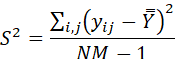
where N denotes the total number of clusters in the population and M denotes the number of elements per cluster. (See W. G. Cochran, Sampling Techniques 3rd edition (Wiley, 1977) for the formulas presented here.) The variance of the sample mean per element,
![]()
where n denotes the sample size, is
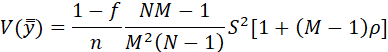
where f = n/N and ρ denotes the intracluster correlation coefficient, defined as
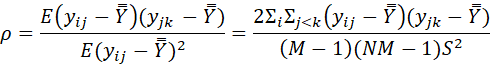
The formula for a sample of nM elements drawn using simple random sampling is the expression on the right-hand-side of the preceding formula preceding the brackets. Hence the bracketed expression, [1 + (M – 1)ρ], indicates how much the variance differs for cluster sampling from the variance for a simple random sample of the same size (nM). This is Kish’s deff for cluster sampling.
If it is assumed that we are sampling clusters from a conceptually infinite population of clusters, then this formula reduces to
![]()
The formula for ρ is a little complicated:
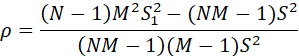
where S12 denotes the variance between unit (cluster) means (note that Cochran uses a slightly different formula, involving the variance, Sb2 between the cluster totals on a single-unit (element) basis). For N large (or assumed infinite), this simplifies to
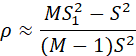
This gives the following approximation for S12 in terms of ρ:
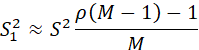
We also have, for N large, the following approximation for S22 in terms of ρ:
![]()
where S22 denotes the within-unit (within-cluster) variance.
Note that ρ can be negative only if M is small. For M large, ρ is approximately equal to S12/S2, which is positive.
In most applications, the values of S12 and S22 are not known, but reasonable assumptions can be made about the value of ρ. If the clusters are relatively internally homogeneous, the ρ is large, e.g., .5 to 1. If units within clusters vary about as much as the general population, then ρ is small, e.g., 0 to .3. The value of ρ is used to estimate the value of deff (in this case equal to (1+(M-1)ρ)), which is entered into the formula (program) for estimating sample size.
For two-stage sampling, where a sample of m elements is randomly selected from each cluster, the formula for the variance of the sample mean per element is
![]()
where f1 = n/N and f2=m/M denote the first- and second-stage sampling fractions, and where S12 denotes the variance among primary unit means and S22 denotes the variance among subunits within primary units:
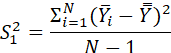
and
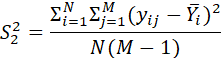
If we assume that N is large, this simplifies to
![]()
If M is large, this simplifies further to
![]()
In terms of the intracluster correlation coefficient, the variance of the sample mean per element is (for N and M large)
![]()
(This expression is obtained by using the approximations (for N and M large) S22 ≈ (1 – ρ)S2 and S12 ≈ ρS2, where S2 was defined earlier.) Since the expression outside of the brackets is the formula for the variance of a simple random sample of size nm, the expression in the brackets shows the change in the variance for two-stage sampling (from simple random sampling), and is hence the (approximate) value of the design effect, deff. In the case of single-stage cluster sampling, the deff, (1 + (M-1)ρ), was defined in terms of M, which is known. Here, the deff, (1 + (m-1)ρ), is defined in terms of the element sample size, m. In order to know the value of deff, m must be specified. We will now show how to do this. (The preceding formula for the deff shows that it increases in direct proportion to m (or M) and ρ.)
As with single-stage cluster sampling, in most applications the variances S12 and S22 are not known, and the value of the intra-unit correlation coefficient is used to determine sample size. For two-stage sampling, however, there are two sample sizes to be determined: the number, n, of first-stage sample units (primary sampling units, PSUs) and the number, m, of elements to select per first-stage unit. We shall consider the case in which a constant number of elements (m) is selected per first-stage unit (this would be appropriate, for example, if the first-stage units were of constant size, or were selected with probabilities proportional to size).
The standard approach to determining the within-unit sample size, m, is to specify a sampling cost function and determine the value of m that minimizes the variance of the estimated mean per element subject to specified cost or that minimizes the cost subject to specified variance. If the cost function is
![]()
then the optimal value of m is

Since the values of the variances S12 and S22 are usually not known, this formula is of limited value. If we use the approximations given earlier for S12 and S22 in terms of ρ (and S2), this formula can be approximated (for ρ not equal to zero) by:
For many applications, this optimum value is rather “flat,” i.e., it is not highly sensitive to small variations in ρ. For many applications, such as sampling households from villages, the number of households is in the range 15-30. Note that the value of mopt is set independently of the value of the first-stage unit sample size, n. Once m has been determined (as mopt), the value of n is then determined by solving the cost equation or the variance equation, depending on whether the cost or the variance has been specified. (Note that if mopt > M or S12 < S22/M, set m = M and use single-stage cluster sampling.)
Now that the value of m is specified, the value of deff, (1 + (m-1)ρ), can be calculated and used in the sample-size formula (program). For many sample surveys in developing countries, villages are primary sampling units (first-stage sampling units) and households (farms) within villages are the ultimate sample unit (second-stage sample unit; element). As mentioned, the number of households per village is often in the range 10-30. If the value of ρ for a variable of interest (e.g., income) is .3 and the value of m is 15, then the value of the deff is 1 + (m-1)ρ = 1 + (15-1).3 = 5.2. That is, the precision associated with sampling of villages is about one-fifth that for simple random sampling. This example shows, as is often the case, that a tremendous loss in precision may result from the use of multistage sampling. The incentive for keeping the village sample size as large as possible is strong.
Sampling from Infinite Populations
It was mentioned earlier that in evaluation research, the finite population correction is not relevant. It is not necessary to use the complicated finite-population formulas involving N and M in evaluation research. These formulas are presented and discussed because they are available in most sample-survey textbooks, which generally deal with descriptive survey design, and because relatively little information is available in textbooks on analytical survey design. This section will discuss some of the fundamental relationships just discussed (for multistage sampling), in the case of sampling from infinite populations (i.e., sample for independent and identically distributed random variables).
The relationship of ρ to S12 and S22 is complicated because of the finite populations. If both N (the unit population size) and M (the cluster size) are large, the formulas become simple, and it is easier to see what is going on. In this case, a simple model of the situation is that the element response is
x = x1 + x2
where x1 denotes the mean of the unit to which the element belongs and x2 denotes a deviation from the mean. Both x1 and x2 are random variables, independent of each other. The value of x1 is independent from unit to unit, and all values of x2 are independent. The mean of the x1 is the population mean, μ, and the mean of the x2 is zero within each unit. Denote the variance of x1 as σ12 and the variance of x2 (the same for every unit) as σ22. Then, by independence of x1 and x2,
var x = var x1 + var x2
where “var” denotes “variance,” or
σ2 = var x = σ12 + σ22
By the definition of ρ, which is
ρ = E (x – μ)(y – μ)/(σ1 σ2)
where E denotes expectation and x and y are two elements in the same unit, it is easy to show that
ρ = σ12 / σ2
and hence σ12 = ρσ2 and σ22 = (1 – ρ)σ2. The formula for the variance of the sample mean, xbar, is
var (xbar) = σ12 / n + σ22 / nm.
Substituting the values for σ12 and σ22 in terms of ρ, we obtain
var (xbar) = (σ2 / nm) (1 + (m – 1) ρ),
which is the approximate expression obtained earlier for two-stage sampling for N and M large.
Determination of the Value of m (the number of second-stage units)
In multistage sampling, there is a sample size for each level (stage) of sampling. In many applications, there are two levels of sampling, for example (in a developing-country context) the selection of a first-stage sample of villages or other primary sampling units (PSUs) and a second-stage sample of households within villages. In this case, there are two sample sizes, which have been denoted in the preceding discussion as n, the number of first-stage sample units, and m, the number of second-stage units.
This section will deal with the problem of determining the number of first- and second-stage units. In general, sample-size estimation programs are used to determine either the total number of first-stage units or the total number of second-stage units. It is assumed that the value of m is known, and whichever is determined, the other is determined accordingly by multiplying or dividing by m. There is a very good reason for this approach (of determining n from m), since it turns out that for analytical surveys the value of m is independent of the value of n. (Usually, the total number of second-stage units is determined by the sample-size-estimation program, and the number of first-stage units (n) is derived from that total by dividing by m.) This section will show why this is true.
To determine the values of n and m, the standard approach is to place a constraint on the total survey cost, and to determine the values of n and m that minimize the variance of the estimated mean. This approach was mentioned above, and approximate expressions were given for the optimal value of m. This section will derive exact expressions, for the infinite-population case (of sampling independent and identically distributed random variables).
We shall assume the same marginal survey cost function as was used earlier, viz.,
C = c1 n + c2 nm .
As was just discussed, the formula for the variance of the estimated mean is
var (xbar) = (σ2 / nm) (1 + (m – 1) ρ) .
What we wish to determine is the values of n and m that minimize the variance, given the constraint on cost. This constrained-optimization problem may be solved by the method of Lagrange multipliers. We form the Lagrangian function
L(n,m,λ) = (σ2 / nm) (1 + (m – 1) ρ) + λ (c1 n + c2 nm – C) ,
and set the partial derivatives with respect to m, n and λ equal to zero, obtaining the following three equations:
-(1 - ρ) σ2/(nm2) + λ c2 n = 0
-(1 + (m – 1) ρ)σ2/(n2m) + λ (c1 +c2m) = 0
c1 n + c2 nm – C = 0 .
Solving the first two for λ and setting the solutions equal, we obtain
(1-ρ) σ2/(nm2c2n) = (1 + (m-1)ρ)σ2/(n2m(c1 + c2m)) .
Solving this equation for m we obtain
mopt = sqrt(c1(1-ρ)/(c2ρ)) .
This is exactly the approximate formula presented earlier, in the case of sampling from finite populations, when M and N were large.
The amazing thing about this result is that it is independent of both C and n. That is, the number of second-stage units to select from each first-stage unit is the same, regardless of C and n. For this reason, the sample-size estimation programs can determine either the number of first-stage sample units (n) or the total number of second-stage sample units (nm), and determine the other by multiplication or division by m.
In practice, the process of determining sample size is an iterative process. In the final analysis, it is usually driven mainly by budgetary considerations. Preliminary sample-size estimates will be made under various assumptions, but they will generally not match the available budget (usually the initial estimates are higher than the budget will accommodate). At this point, the question arises of how to adjust the sample sizes to fit the budget. The answer is that this is done by changing the value of n, and that the value of m remains fixed. This result is counterintuitive. When most people hear it, they do not believe it. They feel strongly that if the sample size can be increased, it would be reasonable to increase both n and m. This is not the case – the value of m depends on the relative survey costs (c1 and c2) and on the intraunit correlation coefficient (ρ), and on nothing else. So, for example, in a two-stage survey of villages and households within villages, the number of households to sample per village will be determined (by specifying c1, c2 and ρ), and then the number of villages will be determined to fit the budget (assuming that it delivers an adequate level of precision or power).
It is noted that the sample-size estimates vary substantially, depending on the values of a number of parameters (effect size to be detected, variances and correlations). In many cases, the values of these parameters are educated guesses. In practice, sample sizes are determined by showing that an adequate level of precision or power can be achieved for a specified sample size that fits the available budget, under a reasonable set of assumptions about the parameters (i.e., a sensitivity analysis is done). The parameters are varied over reasonable ranges, and the sample sizes and power (or precision) examined. Moreover, the assumptions will vary according to the particular outcome variable being considered. It is not the case that there is a single fixed “best” sample-size estimate.
The reason why increases in precision come from increases in the first-stage sample size (n) and not from increases in the second-stage sample size (m) is that the first-stage sample units provide information about the entire population, whereas the second-stage sample units simply provide information about the first-stage units in the sample. There is no point to knowing more and more about a fixed set of first-stage units – there is every reason to want to include additional first-stage units in the sample, to learn more about the total population.
This same phenomenon is manifest relative to estimation of the mean, even in dealing with sampling from finite populations. As noted earlier, the formula for the variance of the mean for two-stage sampling is:
![]() .
.
An unbiased estimate of this is
![]() .
.
where
![]()
and
![]() .
.
If f1 = n/N is small, then the estimated variance may be approximated as
![]() .
.
If n/N is not small, this overestimates by the amount f1S12/n (see Cochran Sampling Techniques 3rd edition (Wiley 1977) pp. 278-79).
There are two interesting features about this result. First, it shows that the variance can be estimated from information about the first-stage means alone. Second, since it does not involve an estimate of the variance of the second-stage means, we do not need to design the second-stage sample to provide this information (i.e., to provide data to estimate the within-first-stage-unit variance). This means that we may employ systematic sampling for the second-stage units (the variance cannot be estimated for a systematic sample, unless it uses more than one random starts). This is often done in two-stage surveys (e.g., forming a list of households in a village, taking a random start, and selecting “every k-th” household for the sample), and it is theoretically justified whenever n is small compared to N. For the infinite-population case (which applied to evaluation research), this assumption applies.
The preceding results show that consideration of the variance of the second-stage units is irrelevant in both design and analysis, for evaluation surveys. This is a direct consequence of the fact that in evaluation surveys, the sample is viewed as being selected from an infinite population, so that the FPC is irrelevant. These results hold approximately for descriptive surveys in which n is small compared to N, but hold exactly for analytical surveys.
Sample-Size Determination for Analytical Surveys; Statistical Power Analysis
There are two main ways of determining sample size in surveys: (1) to determine the sample size required to provide a specified level of precision (e.g., measured by the size of the standard error of an estimate or the size of a confidence interval) for an estimate of a particular quantity (such as a double-difference estimate); and (2) to determine the sample size required to provide a specified power for a specified test of hypothesis (such as the probability of detecting a double-difference of a specified size). The former method is generally used in determining sample sizes for descriptive surveys, and the latter method is generally used for determine sample sizes for analytical surveys. The latter method of determining sample size is usually referred to as “statistical power analysis.” The Brixton program mentioned above determines sample size based on specification of a level of precision; the Statistica program (for example) determines sample size based on specification of power. Depending on how the input parameters are defined and specified, sample-size programs may be used to determine either the number of lowest-level sample units (ultimate sample units; elements), or the number of highest-level sample units (first-stage (primary) sample units). To use these programs effectively, it is necessary to know something about the structure of the population, such as unit and element variances, intra-cluster correlation coefficients, and spatial and temporal correlations. In addition to depending on population characteristics, the sample-size formulas depend crucially on the nature of the sample design. Computer programs for determining sample sizes vary substantially in how much information is specified about the sample design. In some cases, features of the design are explicitly specified, and in others, the effect of design features is implicitly reflected in the value of the design-effect parameter, deff.
The use of techniques recommended for analytical survey designs – panel sampling and matched comparison groups – will cause the design effect for overall-population estimates to be substantially increased. This is not a great concern, for the objective in analytical surveys is to estimate differences and relationships, not overall population characteristics (means and totals). The deff refers to the increase in the variance of the estimated mean (or total) over that achieved with simple random sampling (of the same ultimate-unit sample size), not to the ratio of the variance for a difference or double difference. (It would be clearer if the estimate to which a design effect corresponds were always explicitly identified, but this is usually not done – it usually refers (without mention) to the population mean or total.)
The formulas used to estimate sample sizes for descriptive surveys should not be used to estimate sample sizes for analytical surveys – they do not explicitly reflect the features that are present in analytical survey designs (panel sampling, matching of comparison groups), nor do they account for the fact that the estimates of interest are differences (or double differences), not overall population characteristics.
Theoretically, it may be possible to use the descriptive-survey formulas for determining sample sizes for analytical surveys, but in practice the designs are so complex that it is not possible to estimate a reasonable value for the deff. (A typical analytical survey design for an impact evaluation will include not only stratification, multistage sampling and selection of units with variable probabilities, but also panel sampling and construction of comparison groups by matching of individual units.) What is needed is a sample-size estimation procedure that takes into account the special features of an analytical survey design, such as panel sampling and construction of comparison groups by matching of individual units.
As mentioned, the principal method of determining sample sizes for analytical surveys is statistical power analysis. The emphasis is on power (rather than precision) since analytical surveys are involved with tests of hypothesis – descriptive surveys are concerned mainly with precision of estimates, not with the power of tests of hypothesis. Consideration of power is a fundamental aspect of the branch of statistics known as “testing statistical hypotheses.” This is a very old branch of statistics. The fundamental theorem of hypothesis testing is the “Neyman-Pearson Lemma,” which states necessary and sufficient conditions for a most powerful test of an hypothesis. This theorem was proved in the 1920s. (The major reference book on testing statistical hypotheses is Testing Statistical Hypotheses by E. L. Lehmann (Wiley, 1959, 2nd edition 1986). This is a “companion” to Lehmann’s book on point estimation, Theory of Point Estimation (Wiley, 1983).) There are two parameters that may be specified for a test: the probability of making a Type I error, or rejecting a null hypothesis when it is true (this probability is called the “size” or “significance level” of the test, and is usually denoted by α); and the probability of making a Type II error, or accepting a null hypothesis when it is false (this probability is usually denoted by β). The power of the test is the probability of rejecting the null hypothesis, or 1 – β. In general, power analysis should address both the values of α and β, but it is customary to do power calculations for “standard” values of α, such as .0005, .01 or .05. (This tradition stems from the early days of statistics, prior to computers, when much use was made of hard-copy tables, which were constructed only for a limited set of values of parameters of interest.)
The probability of rejecting a null hypothesis depends on which alternative hypothesis is true. In many applications, the null hypothesis is that a parameter (such as a mean or a double-difference) has a particular value, and the alternative is that the parameter differs from this value by a specified amount, D. In this case, the power of the test may be considered as a function of the value of D. This function is called a “power function,” or “power curve.” The power curve is the probability of rejecting the null hypothesis as a function of D. The one-complement of the power function, or the probability of accepting the null hypothesis as a function of D, is called the “operating characteristic” curve (or “OC” curve).
Descriptive surveys are concerned with estimation, and analytical surveys are concerned with hypothesis testing. Here follows a quotation from Introduction to the Theory of Statistics by Mood, Graybill and Boes (McGraw-Hill, 1963, 3rd edition 1974): “The power function will play the same role in hypothesis testing that mean-squared error played in estimation. It will usually be our standard in assessing the goodness of a test or in comparing two competing tests. An ideal power function, of course, is a function that is 0 for those θ corresponding to the null hypothesis and is unity for those θ corresponding to the alternative hypothesis. The idea is that you do not want to reject Ho if Ho is true and you do want to reject Ho when Ho is false.” [The parameter θ specifies a probability distribution; Ho denotes the null hypothesis. Mean-squared error is variance plus the square of the bias.]
All basic-statistics books include discussions of the power of statistical tests of hypothesis. Consideration of power is a central focus of the field of statistical quality control (through plots of its one-complement, the probability of accepting the null hypothesis, via the operating characteristic curve). See, for example, Quality Control and Industrial Statistics by Acheson J. Duncan (Irwin, 1952, revised edition 1959, 5th edition 1986). It is a curious fact, however, that consideration of power is largely absent from older books on sample survey. For example, the classic text, Sampling Techniques 3rd edition by W. G. Cochran (Wiley, 1977) does not even include the word “power” in the index. Nor does Elementary Survey Sampling 2nd edition by Scheaffer, Mendenhall and Ott (Duxbury Press, 1979). Nor do any of the other older major texts on sampling. There is, of course, a reason for this: these texts deal with descriptive surveys, and descriptive surveys are concerned with estimation, not with tests of hypothesis. What is quite amazing, however, is that even recent sampling texts, such as Lohr’s, Thompson’s, and Lehtonen/Pahkinen’s, do not address the topic of statistical power analysis.
In recognition of the fact that books on sample survey did not consider power, Jacob Cohen wrote the book, Statistical Power Analysis for the Behavioral Sciences (Academic Press, 1969). This book is of little relevance to the field of sample survey, however, since it deals exclusively with simple random sampling.
The Role of the Significance Level of a Statistical Test of Hypothesis
The determination of sample size by specifying precision of an estimator involves specification of two factors: the level of precision desired (e.g., as specified by the magnitude of the standard error of an estimate or by the width of a confidence interval of a prescribed confidence coefficient (such as 95 percent)) and the variability of the population. The determination of sample size by specifying the power of a test of hypothesis involves specification of four factors: the magnitude of the effect size to be detected, the significance level of the test (probability, or size, of the Type I error), the level of power (probability of rejecting the null hypothesis, i.e., of detecting the effect), and the variability of the population.
The relationship between the significance level and the power is very important, and it is often overlooked. Here follows a quote from Lehmann’s Testing Statistical Hypotheses, 2nd edition (Wiley, 1986, pp. 69-70): “The choice of a level of significance α will usually be somewhat arbitrary, since in most situations there is no precise limit to the probability of an error of the first kind that can be tolerated. Standard values, such as .01 or .05, were originally chosen to effect a reduction in the tables needed for carrying out various tests. By habit, and because of the convenience of standardization in providing a common frame of reference, these values gradually became entrenched as the conventional levels to use. This is unfortunate, since the choice of significance level should also take into consideration the power that the test will achieve against the alternatives of interest. There is little point in carrying out an experiment which has only a small chance of detecting the effect being sought when it exists. Surveys by Cohen (1962) and Freiman et al. (1978) suggest that this is in fact the case for many studies. Ideally, the sample size should then be increased to permit adequate values for both significance level and power. If that is not feasible, one may wish to use higher values of α than the customary ones. The opposite possibility, that one would like to decrease α, arises when the latter is so close to 1 that α can be lowered appreciably without a significant loss of power (cf. Problem 50). Rules for changing α in relation to the attainable power are discussed by Lehmann (1958), Arrow (1960), and Sanathanan (1974), and from a Bayesian point of view by Savage (1962, pp. 64-66). See also Rosenthal and Rubin (1985).”
The reason why there are so many “false alarms” of studies that claim to show the efficacy of some medicine, later to be discredited, is more likely to be the result of the setting of the significance level much too low, e.g., .05, than of a faulty research design. At the .05 level, there is a one-in-twenty chance that the study will show a “significant” effect, simply by chance, when there is none. It would appear that it would be much more cost-effective for socio-economic studies to use much higher levels of α, such as .001 or .0001. The increased risk that this carries that some positive effects may be unnoticed is not very troubling, since these “missed” effects will be small. On the other hand, program managers do not want to see results that suggest that their programs are not effective, even if the effect is very small. So they will press for large values of α, such as .05, in program evaluation studies. (This will mean that “significant” results will be concluded, even when they are not true, about five percent of the time.) This accrues the additional advantage to the program manager of allowing smaller sample sizes (since if α is higher, the power is also higher for the same sample size; or, if α is higher, the sample size required to achieve a specified level of power is lower).
Computer Programs for Determining Sample Size for Analytical Surveys
Recently, funded by a grant from the William T. Grant Foundation, researchers at the University of Michigan conducted a project to develop computer software to conduct statistical power analysis. A report describing their work is Optimal Design for Longitudinal and Multilevel Research: Documentation for the “Optimal Design” Software, by Jessaca Spybrook, Stephen W. Raudenbush, Richard Congdon and Andrés Martinez, University of Michigan, July 22, 2009. The report and the software are posted at http://sitemaker.umich.edu/group-based/home or http://sitemaker.umich.edu/group-based/optimal_design_software. This software conducts statistical power analysis for a variety of sample designs, for randomized trials. Since randomization is used to assign treatment level to experimental units (the authors assume two treatment levels – treatment and control), the treatment and control groups are “statistically equivalent” (i.e., have the same joint distribution for all variables other than treatment), and a comparison between the treatment and control groups may be made with a single-difference estimate, rather than the double-difference estimate between these two groups at two different points in time. The Optimal Design software produces a wide range of output.
Another program for determining sample size for survey designs in evaluation (i.e., for analytical surveys) is available at the author’s website, http://www.foundationwebsite.org/SampleSize.exe . The program determines the sample size of primary sampling units. It calculates sample sizes for a number of cases involving differences in means of population subgroups, including the “double difference” estimator. This program considers three different survey designs – random sampling of primary sampling units for estimation of a population mean; random sampling of two groups, for estimation of a difference in group means (a “single difference”; and random sampling of four groups, for estimation of a double-difference in group means. This last case corresponds to the “pretest-posttest-with-comparison-group” design that is often used (either as an experimental design (randomized comparison group) or quasi-experimental design) in evaluation research. In addition to specifying parameters for the design (such as means, variances and correlations), the user may specify a value for a design effect (deff). The deff is intended to address all design features that are not already addressed by the specified design structure and parameters. For example, in the case of the four-group design, the various correlation coefficients requested would take into account correlations introduced by matching and by panel sampling, and the deff would take into account all other design effects (e.g., caused by stratification or multistage sampling).
It is emphasized that the formula for calculating sample size depends both on the estimate of interest and on the sample design. The most common design in evaluation studies is a pretest-posttest-with-comparison-group design. The author’s sample-size program calculates sample sizes for this design (and simpler designs).
Single-Difference vs. Double-Difference Estimators
An interesting issue that arises with evaluation designs is the following. Suppose that the objective is to estimate the change in income caused by a certain program, and that the treatment groups and control groups are determined by randomization (i.e., randomized assignment of treatment level (treatment or control) to units). In this case, the treatment and control groups are equivalent with respect to all variables except treatment level. Hence, they are equivalent at the beginning of the evaluation, and the impact of the program intervention may be estimated simply by calculating the difference in income means between the treatment and control groups at the end of the study. The interesting thing, however, is that if pretest and posttest data are available, most analysts would still use the double difference in means (difference, before and after the study, between the difference in means of the treatment and control groups) to estimate program impact. It is important to understand why this is so.
Ordinarily, with independent simple random sampling of four groups, it would be advantageous to use a single difference instead of a double difference because (as will be discussed later) the variance of a double difference is four times as large as a single difference based on the same number of observations. Because of the introduction of correlations between the treatment and control groups (introduced by use of matched pairs) and the before and after groups (introduced by use of panel sampling), this factor of four could be reduced substantially, in many cases to the point where the double-difference estimate may even be more precise than the single-difference estimate. This, however, is not the reason for using the double-difference estimator. There are several reasons for doing so.
First, when matching is done, it is usually done on clusters (aggregates, higher-level sample units), such as villages, districts, census enumeration areas, or other administrative units. The reason for this is that data required for ex ante matching are known (prior to the survey) usually only for aggregates, not for the ultimate sample unit of interest (such as a household). The typical design, then, is a multi-stage design, in which the number of primary sampling units is usually not very large. It could be as large as 100 or more, or it could be as few as five or ten. For small sample sizes, however, the two fundamental theorems so frequently invoked in statistical analysis – the law of large numbers (which says that for large samples the sample mean is close to the population mean) and the central limit theorem (which says that for large samples the sample mean is approximately normally distributed) – do not apply. For a small sample of PSUs, it is quite possible for the treatment group and the control group to be rather different. For example, the means with respect to one or more variables could be somewhat different. In other words, the particular samples selected for the treatment and control groups might not be highly “orthogonal” (conditionally independent) with respect to some variables (observed or unobserved). (The theory of propensity-score matching, for example, relates to asymptotic (large-sample) properties of the matching process – it does not apply well for small sample sizes.) In this case, although the sample estimates are unbiased in repeated sampling, the particular sample may provide poor results, simply because it is small (the “luck of the draw”), not because the randomization process was flawed. A way to improve the precision of the estimator is to use a double difference estimator instead of a single difference estimator. The reason the double difference estimator performs better is because it is based on matched pairs with matching not only between both treatment and controls, but also between pretest and posttest units (via panel sampling). The double difference estimator is a more complex “model-based” estimate than the single difference estimator, and less sensitive to vagaries of sample selection. (In fact, for a correctly specified model, we do not need a probability sample at all – just a sample with good spread, balance and orthogonality on all variables of interest.)
The second reason why a double difference estimator would be used even for a design involving randomized selection of treatment and control groups is nonresponse. If some PSUs are “lost” from the sample (e.g., refusal to participate in the survey, lack of access due to rain, outbreak of disease (quarantine) or civil disturbances), it is usually desirable to substitute replacements for them, to maintain the sample size (in a matched-pairs design, both units of a matched pair should be replaced, if practical, when either one of the pair is replaced). While this may keep the precision level high, it may also introduce selection bias (if the outcome is in some way different for the nonresponders). In this case, we do not have the pure experimental design that we had planned. The double-difference model is less sensitive to selection bias than the single-difference model, for the same reason as discussed above.
In summary, for a pretest-posttest-with-randomized-control-group design, a double-difference estimator is used, even though a single-difference estimator is correct (conceptually appropriate). The single-difference estimator would be used only if baseline (pretest, time 1) data were not available. (A double difference estimate of impact would always be used for a quasi-experimental pretest-posttest-with-comparison-group design, since there is no guarantee that the treatment and control groups are equivalent – they can be matched only on observables.)
The Importance of Correlation in Analytical Survey Designs; Estimation of Differences
As is clear from the preceding discussion, the determination of sample size for analytical surveys proceeds quite differently for analytical surveys than for descriptive surveys. Sample size determination for descriptive surveys generally focuses on specification of the level of precision for an estimator (such as a population mean or total), whereas for analytical surveys it focuses on specification of the power for tests of hypotheses (such as whether two populations could be considered to have the same probability distribution (or mean)).
There is another very significant difference. In order to calculate sample size for analytical surveys, it is essential to know something about the correlation between observations in different groups involved in estimates of interest. For example, the double-difference estimate of program impact for a pretest / posttest / comparison-group design involves a double difference (linear contrast) of four groups – the treatment and comparison groups before the program intervention (pretest) and these two groups after the program intervention. In a descriptive survey, the observations of four different population subgroups (e.g., four different strata) would typically be uncorrelated (i.e., be selected independently of each other) – this would maximize the precision of estimates of means and totals. In an analytical survey, the observations involved in an estimate of interest (such as the double difference) would almost certainly be correlated, by intention (i.e., by design). The reason for introducing correlations among the four groups is to increase precision (via a “matched pairs” sample that includes matching of individual treatment units with individual control units, and individual time-1 units with individual time-2 units). In the example just mentioned, the survey designer would prefer to use a panel survey involving reinterview of the same sample units before and after the program intervention. This would dramatically increase the precision of the double-difference estimate, over the case in which the units of the second round of the survey were independently selected. Also, the survey designer would prefer to promote local control between the treatment and comparison groups by matching individual units (or “blocking”), rather than simply matching the probability distributions (i.e., by using unrelated (independent) samples). This would have a large impact on the precision of the estimate, depending on how effective the matching was in reducing the variation between paired treatment and comparison units.
To take the effect of panel sampling and matching of treatment and comparison units into account, it is necessary to specify the correlation between panel units and the correlation between treatment and comparison units. A simple example will illustrate the concept involved. Suppose, for example, that we wish to use a sample to estimate the overall population mean, and also to estimate the difference between two population subgroups. If the samples for the two subgroups are selected independently (e.g., strata in a descriptive survey), then the formulas for the variance of the estimated mean and difference are
var(mean) = var (![]() +
+ ![]() )/2 = (1/4) (var
)/2 = (1/4) (var ![]() + var
+ var ![]() ) = (1/4) (v1/n1
+ v2/n2)
) = (1/4) (v1/n1
+ v2/n2)
var (difference) = var (![]() -
- ![]() ) = var
) = var ![]() + var
+ var ![]() = v1/n1
+ v2/n2
= v1/n1
+ v2/n2
where
![]() v1 and v2
denote the within-stratum variances of units and n1 and n2
denote the stratum sample sizes. If v1 = v2 = v (i.e.,
the strata are no more internally homogeneous than the general population, so
that stratification is of no help in reducing the variance) and n1 =
n2 = n/2 (a “balanced” design), then these estimates become
v1 and v2
denote the within-stratum variances of units and n1 and n2
denote the stratum sample sizes. If v1 = v2 = v (i.e.,
the strata are no more internally homogeneous than the general population, so
that stratification is of no help in reducing the variance) and n1 =
n2 = n/2 (a “balanced” design), then these estimates become
var(mean) = v/n
var(difference) = 4v/n,
which are the usual formulas for the variance of the mean and difference in the case of simple random sampling. These formulas illustrate that for descriptive surveys (independent sampling in different strata) four times the sample size is required to produce the same level of precision (as measured by the variance (or its square root, the standard deviation) for an estimated difference as for an estimated mean – a sample of size 2n is required for each of the two groups (strata) comprising the difference, instead of a single sample of size n overall.
(This may seem a little counterintuitive. If a sample size of n is required to produce a certain level of precision for an estimated population mean, then that same sample size is required to produce that level of precision for a subpopulation mean (assuming that the variance of the subpopulation is the same as the variance of the general population). Hence the sample size required to produce comparable-precision estimates of two subpopulation means, each equal in size to half the population, would be 2n (i.e., n for each subpopulation). The variance of the difference in these two means, however, is twice the variance of each individual mean. Hence, to obtain the same level of precision for the estimated difference, the sample size must be doubled again, to 2n for each group.)
If steps are taken to pair similar items, such as in panel sampling (reinterview of the same unit at a later time) or matching of individual treatment and comparison units, then the sample items represent “paired comparisons,” and the variances of the estimated mean and difference change. If ρ denotes the correlation coefficient between the units of matched pairs, then
var(mean) = (1/4) {v1/n1 + v2/n2 + 2 ρ sqrt[(v1/n1)(v2/n2)]}
var(difference) = v1/n1 + v2/n2 - 2 ρ sqrt[(v1/n1)(v2/n2)].
What we see is that the presence of correlation between paired units increases the variance of the mean and decreases the variance of the difference. In analytical surveys, we are generally interested in estimating differences (or regression coefficients, which are similar), and so the presence of correlations between units in different groups involved in the comparison can reduce the variance of the estimate very much. If v1 = v2 = v and n1 = n2 = n/2, these formulas become
var(mean) = (1 + ρ) v/n
var (difference) = (1 – ρ) 4v/n.
For example, if ρ = .6, then the variance of the mean is 1.6 v/n and the variance of the difference is also 1.6 v/n. Because of the introduced correlation, the standard deviation of the difference has been reduced by a factor of sqrt(1.6/4) = .63 and the standard deviation of the mean has been increased by the factor sqrt(1.6/1) = 1.26.
In designing an analytical survey, it is differences rather than means (or proportions or totals) that are of primary interest, and the survey designer will construct the design so that the correlations between units in groups to be compared are high. For estimating a double difference, the two correlations of primary interest are the correlation between corresponding units of the panel survey and the correlation between matched treatment and comparison units. (The presence of these correlations will introduce correlations among other groups, e.g., between the pretest treatment group and the posttest comparison group. These correlations affect the variance of the estimates, but they are not of direct interest, and are not controlled. This will be discussed in greater detail later.)
Keep in mind that while the introduction of correlations (via matching and panel sampling) will improve the precision of double-difference estimates, it will reduce the precision of estimates of population means and totals. In many survey applications, it is desired that the survey be capable of producing both kinds of estimates, and so the design will be a compromise between (or combination of) a descriptive survey and an analytical survey (or between the design-based approach and the model-dependent approach, i.e., it will be a model-based approach). A practical example is a sample survey designed to produce data for both program monitoring and evaluation (“M&E”). For program monitoring, primary interest focuses on estimation of means and totals for the population and for various population subgroups. For impact evaluation, attention focuses on estimation of differences (comparisons, linear contrasts, regression coefficients). From the viewpoint of efficiency, it would appear to be desirable to address both concerns simultaneously, i.e., not to design a monitoring system based on one survey design and then have to develop a separate design for impact evaluation. In a monitoring and evaluation application, the monitoring system is an example of a descriptive survey, and the impact evaluation is an example of an analytical survey, but both surveys involve the same population over the same time period, and so it is desirable from an efficiency viewpoint to address both objectives simultaneously.
Although it may appear to be efficient to use the same sample designs and sizes for both monitoring and evaluation, appropriate (“efficient”) designs and sizes are so very different for these two settings that it does not make much sense to try to address them both with the same survey. In a monitoring setting, the questionnaires are usually brief, the sample sizes very large (often all of the clients), and the data collected by a service provider. In an evaluation setting, the questionnaires are usually lengthy, the sample sizes are usually smaller, and the data collected by a trained interviewer. In the monitoring setting it is usually desired to obtain estimates of overall population characteristics, but no attempt is made to obtain a statistically rigorous estimate of program impact. As mentioned, the (descriptive) survey designs for estimating overall population characteristics are quite different from the (analytical) survey designs for estimating program impact. The presence of correlations that make the impact (difference) estimates precise cause the precision of monitoring estimates (overall population characteristics such as means and totals) to be very low. Finally, monitoring systems typically involve storage of data for all clients in a relational database management system (such as Microsoft Access). Whenever an estimate is desired, it can typically be produced using data for the complete population – there is no need for statistical estimation or hypothesis testing.
One area in which it is advantageous to coordinate the design of the monitoring system and the evaluation study is in the specification of variables to be observed. In monitoring and evaluation, the dependent variables are usually referred to as “indicators” or “measures of performance.” In most evaluation settings, the monitoring system is developed (designed and set up) when the program starts, and the evaluation study is constructed (designed and implemented) later (e.g., near the end of a multi-year program). It is advantageous if sufficient coordinated thought can be put into the design of both systems, at the beginning of the program, so that the dependent variables and the independent variables “overlap,” in the sense that if a variable is useful for both systems, it has the same definition. This way, it may be possible to combine the monitoring data with the evaluation data to construct improved estimates.
The distinction between outcome and impact measures was mentioned earlier. Monitoring systems are concerned with measurement of outputs (e.g., trained farmers) and outcomes (e.g., increased income, better access to educational services), whereas an evaluation study is concerned with impact (e.g., a double-difference estimate of income).
The sample-size program posted at the author’s website addresses the problem of determining sample size to estimate the double-difference of a pretest / posttest / comparison-group design, but it does not address more complex designs, such as an application involving multiple comparison groups. Such cases would involve forming matched “groups” rather than matched pairs, to improve the precision of comparisons among several groups, not just two. The matching methodology presented in Appendix A addresses the issue of constructing matched groups, as well as matched pairs.
Note that the “deff” referred to in the sample-size program is the design effect corresponding to design aspects other than those reflected in the correlations between the treatment and control groups, and between the pretest and posttest groups. (Furthermore, as discussed earlier, it is the deff corresponding to the estimation of means and totals, not of differences or double differences.) The deff to be specified should reflect the design effect from other design features, such as stratification, clustering, multistage sampling and selection with variable probabilities, not the specified correlations (among the four groups).
Sample-Size Determination When Explanatory Variables Are Involved; Simple Models (Analysis of Variance, Analysis of Covariance; Regression)
This section (on sample size) will close with some additional discussion of considerations in determination of sample size, in the case in which it is desired to construct a model that emphasizes comparison of treatment and nontreatment groups, but also includes a number of other explanatory variables. This kind of model is appropriate, for example, when it is not possible to use a true experimental design with randomized selection of the controls (nontreatment units), and a quasi-experimental design is being used as an alternative. Because of the lack of randomization, data are also collected on a number of other variables (in addition to the treatment variable) that may have had an influence on selection for treatment or may have an effect on outcomes of interest. The purpose of constructing the model is twofold: to estimate the relationship of impact to explanatory variables to which it is related, and to adjust an impact estimate for difference (in covariates) between the treatment and control groups and the before and after groups. (The adjustment process is in fact equivalent to estimating the response for a counterfactual.) (The discussion in this section is a little technical, and may be skipped with little loss in the conceptual issues discussed in this article.) (It is noted that data may be collected on nontreatment variables (covariates, explanatory variables) even if randomization is employed, to estimate the relationship of treatment effects to these variables.)
We assume that the model is a general linear statistical model, such as a multiple regression model, an analysis-of-variance model or an analysis-of-covariance model. We first consider the case in which there is a single explanatory variable in the model, viz., the treatment variable. We assume that the design is “balanced,” so that half the observations are treatment units and half are nontreatment units. Denote the sample size as n.
It
was shown earlier that if simple random sampling is used and sampling is done
independently in different groups, the number of observations required to
produce a given level of precision for estimation of a difference in means is
four times that required to produce the same level of precision for estimation
of the overall mean. Let us assume that we have a sample of n independent
observations sampled from a distribution having mean μ and variance σ2.
Let us denote the dependent variable of interest as y. Then the variance of
the sample mean, ![]() , is
, is
var(![]() ) = σ2/n
) = σ2/n
and
the variance of the estimated difference, ![]() 1 -
1 - ![]() 2, is (because of
independence)
2, is (because of
independence)
var(![]() 1 -
1 - ![]() 2) = var(
2) = var(![]() 1) + var(
1) + var(![]() 2) = σ2/(n/2)
+ σ2/(n/2) = 4 σ2/n .
2) = σ2/(n/2)
+ σ2/(n/2) = 4 σ2/n .
We see, as noted earlier, that the variance of the estimated difference is four times the variance of the estimated mean. Similarly, the number of observations required to produce a given level of precision for estimation of a double difference in means is sixteen times that required to produce the same level of precision for estimation of the overall mean, in the case of simple random sampling and independent groups:
var(![]() 1 -
1 - ![]() 2 +
2 + ![]() 3 -
3 - ![]() 4) = var(
4) = var(![]() 1) + var(
1) + var(![]() 2) + var(
2) + var(![]() 3) + var(
3) + var(![]() 4)
4)
= σ2/(n/4) + σ2/(n/4) + σ2/(n/4) + σ2/(n/4) = 16 σ2/n .
(It should be noted that a double difference is not a linear contrast. A linear contrast is a linear combination of the observations such that the sum of the coefficients is zero and the sum of the positive coefficients is one. For all linear contrasts having coefficients of equal magnitude (for each observation), the variance of the linear contrast is equal to 4 σ2/n. For a double difference, the coefficient of each observation is plus or minus 1/(n/4), and the sum of the positive coefficients is (n/2)(1/(n/4)) = 2, not one. A double difference is hence twice the value of such a linear contrast, and so its variance is four times as large, or 16 σ2/n instead of 4 σ2/n.)
Hence we see that if we are comparing independent subgroups, the sample sizes required to estimate differences and double differences become very large. The way that the sample size is reduced to reasonable levels is by avoiding the use of independent groups, by introducing correlations between members in different groups. For estimation of a double difference from a pretest / posttest / control-group design this may be done by reinterviewing the same unit in the posttest (second round of a panel survey) and matching individual control units with treatment units. To keep the example simple, let us see what effect this has in the case of estimating a single difference (the more complicated case of a double difference is considered in the sample size estimation program mentioned earlier, and in an example presented later in this article).
In this case, the formula for the variance of the estimated difference is
var(![]() 1 -
1 - ![]() 2) = var(
2) = var(![]() 1) + var(
1) + var(![]() 2) – 2 cov (
2) – 2 cov (![]() 1,
1, ![]() 2) = var(
2) = var(![]() 1) + var(
1) + var(![]() 2) – 2 ρ sqrt(var(
2) – 2 ρ sqrt(var(![]() 1) var(
1) var(![]() 2))
2))
= σ2/(n/2) + σ2/(n/2) – 2 ρ sqrt(σ2/(n/2) + σ2/n/2)) = 4 (1-r) σ2/n ,
where
cov denotes the covariance of ![]() 1and
1and ![]() 2 and ρ denotes the
correlation of
2 and ρ denotes the
correlation of ![]() 1 and
1 and ![]() 2. That is, the
variance is reduced by the factor (1-ρ). By doing things such as
reinterviewing the same sample unit in the posttest and matching of individual
comparison units with treatment units, the correlation, ρ, may be quite high,
such as .5 or even .9. That is, the variance of the estimated difference may
be substantially reduced.
2. That is, the
variance is reduced by the factor (1-ρ). By doing things such as
reinterviewing the same sample unit in the posttest and matching of individual
comparison units with treatment units, the correlation, ρ, may be quite high,
such as .5 or even .9. That is, the variance of the estimated difference may
be substantially reduced.
In a laboratory or industrial experiment, there may be many treatment variables of interest, and it is important to use a design in which they are orthogonal, such as a factorial or fractional factorial design, so that the estimates of the treatment effects will be uncorrelated (unconfounded) and readily interpreted. In many socioeconomic experiments, there is but a single treatment effect, viz., the effect of program intervention (e.g., increased earnings or employment from participation in a farmer training program, or decreased travel time or cost from a roads improvement program). In a laboratory experiment, there are usually several treatment variables and no covariates, whereas in an evaluation of socioeconomic programs there is often a single treatment variable and lots of covariates. Whichever is the case, it should be realized that differences in many variables may be represented in and estimated from the same data set. The greater the degree of orthogonality among the explanatory variables (i.e., the lower the correlation), the lower the correlation among the estimated effects, and the easier it is to interpret the results.
It is noted that in a well designed experiment is it possible to estimate the effects of a number of treatment variables simultaneously. All that is required is that the number of observations be substantially larger than the total number of effects (linear contrasts) to be estimated (main effects, first-order interactions, second-order interactions, etc.). In many social or economic evaluations, there is only a single treatment variable, viz., participation in the program, but even if there are numerous program variations, it may be possible to evaluate all of them simultaneously, in a single sample (experiment), without the need for separate samples for each treatment variable. If a standard descriptive-survey approach were adopted in this situation, a separate sample (or stratum) might be used for each treatment combination of interest, and a large sample size would be required. This “one-variable-at-a-time” approach would be an inefficient approach, compared to a sample design that addresses multiple treatment combinations at the same time (such as a fractional factorial design).
Estimation of a regression coefficient in a multiple regression model is analogous to estimation of a difference in group means in an analysis of variance (experimental design) model. This is easy to illustrate in the case of an experiment in which there is a single explanatory variable and there are just two values of the variable (e.g., treatment and control). We showed above the formula for the variance of the difference in means between the two groups. For the regression equation, the model is
yi = α + β xi + ei
where α denotes the intercept, β denotes the slope, and e is an error term (independent of each other and the x’s, with mean zero and common variance σ2). The variances and covariance of the estimated parameters (a and b) are:
var(a) = σ2 Σ xi2
/ (n Σ (xi – ![]() )2 )
)2 )
var(b) = σ2 / Σ (xi – ![]() )2
)2
cov(a,b) = - σ2 ![]() / Σ (xi –
/ Σ (xi – ![]() )2 ,
)2 ,
where Σ denotes summation.
Let us define the values of the x’s so that their mean is zero and their range is one (so that the slope coefficient denotes the mean change in y per unit change in x), that is, xi = ½ for treatment units and xi = -½ for nontreatment units (controls). In this case, the three preceding quantities become
var(a) = σ2 /n
var(b) = 4 σ2/n
cov(a,b) = 0.
In this simple regression model, the intercept is simply the overall mean, and the slope is the average difference between the treatment and control groups, and we see that the variances of these two estimates are exactly what we obtained earlier.
In a laboratory experiment, we could have many other treatment variables orthogonal to (uncorrelated with) the first treatment group, and the results would be the same for all of them. As mentioned, in socioeconomic experiments (such as program evaluations), there is usually a single treatment variable, but there may be many additional covariates. The covariates will in general not be orthogonal to the treatment variable, even if we apply the survey design algorithm of Appendix A to reduce the correlation among the explanatory variables.
Let us now examine the variance of certain estimates of interest. The estimate corresponding to a specified value of x is obtained simply by substituting the value of x in the estimated regression equation, y = a + bx. Its variance is given by
var(y | x) = var(a + b x) = var(a) + x2 var(b) – 2 cov(a, bx) = var(a) + x2 var(b)
since the covariance is zero. (See Alexander Mood, Franklin A. Graybill and Duane C. Boes Introduction to the Theory of Statistics (3rd edition, McGraw-Hill, 1974) for the formulas for the variances and covariances of the regression-model estimates.) To estimate the overall mean, substitute x = 0, obtaining y = a and
var(y | x=0) = var(a) = σ2/n.
To estimate the value for the treatment, substitute x = ½, obtaining y = a + ½ b and
var(y | x = ½) = var(a) + ¼ var(b) = σ2/n + ¼ 4 σ2/n = σ2/(n/2).
Note that this is exactly the same as the variance of the estimate of the mean of a sample of size n/2, which is what the set of treatment observations is. In other words, as had to be the case, the use of a regression model to estimate the treatment effect produces exactly the same result as estimating the effect from an analysis-of-variance model, i.e., as the mean difference between the treatment and nontreatment units (difference in means of the treatment and nontreatment groups).
This simple example illustrates well the fact that the variance of an estimator from a regression model depends very much on the value of the explanatory variable, and that estimates for extreme values of x, at the limit of the observation set, such as for the treatment group (treatment value x = ½), will be much lower than the variance for observations near the middle of the observation set, such as the overall mean (treatment value 0). The regression model does not “add” any information to the estimation process, over that reflected in the simple difference-in-means model.
(In sample survey, an improved estimate of an overall population characteristic (such as a mean or total) derived from a regression model is called a “generalized regression estimate” or “GREG” estimate. It is called “generalized” since it is a generalization (extension) of the usual regression or ratio estimation procedure (which typically involves a single regressor (explanatory variable). In evaluation research, a regression model would typically be used to determine an improved estimate of a difference estimator such as a double-difference estimate of program impact, or it could be used to show the relationship of impact to explanatory variables. It would typically not be used (in evaluation research) to determine improved estimates of population means or totals, because the design is configured to estimate differences or double differences, not means or totals. Instead, in evaluation research, the regression model would be used to describe the relationship of impact to explanatory variables, or to adjust the double-difference estimate of impact for differences among the four groups of the pretest-posttest-control-group design (i.e., adjustment for covariates; estimation of counterfactuals). The use of the term “improved” here (in an evaluation study) refers to adjustment for differences (in covariates) between the treatment and control groups. In descriptive sample survey, the term “improved” would be referring to an improvement of the regression or ratio estimate over a simple expansion-type estimate.)
The examples presented above concern independent groups (treatment and control). If we introduce correlations into the design, e.g., by matching of individual units in the treatment and nontreatment groups, the formulas for the variances change. The variance of a will increase by the factor (1 + ρ) and the variance of b will decrease by the factor (1 – ρ), where ρ denotes the correlation between a unit in the treatment group and its corresponding (matched unit) in the comparison group. Note that the estimate of the mean for the treatment group (or the nontreatment group) will still be the same (since the +ρ will cancel the –ρ in the formula). That is, the introduction of correlations between the treatment and nontreatment groups (whether we match the group or match individual items) does not reduce the precision of each estimated group mean.
For a treatment variable having only two values (½ and -½), both values are extreme, and the variance of the group means will be relatively large (compared to that for a central value of x). For variables that have many values over a range, this may not the case. For example, suppose that we wish to estimate a model for four different regions. There are two approaches to doing this. On the one hand, we may select independent samples and estimate separate models for each one. On the other hand, we may posit an overall model for the entire population and reflect differences among the regions by interaction terms in this overall model. This may be a much more efficient use of the data, since data from all four groups is being used to estimate the various model parameters (in a single, combined model). It should be remembered, however, that the process of matching across groups will generally increase the precision of estimates of model parameters and differences at the expense of decreasing the precision of the estimate of the overall mean. In general, the precision of the estimates of the group means will be unaffected by matching across groups. (The precision of estimates of group means will be adversely affected, of course, by any matching done within the groups, such as between units in a treatment and control group).
Although this article is not concerned with estimation, it is noted that the usual formulas for estimation of variances and tests of hypothesis about regression models assume a simple random sample. Because of the complex structure of an evaluation research design (pretest-posttest-comparison-group with panel surveying and matching of treatment and control groups or individual units (matched pairs), the sample is not at all a simple random sample. The general linear statistical model still applies, but the correlation matrix is not and identity matrix (or diagonal matrix or “nicely” structured nondiagonal matrix). In general, estimation (of model parameters and variances) would be done using resampling (pseudoreplication) methods.
Additional Comments on Sample-Size Determination; More Complex Models Involving Explanatory Variables
This section discusses some additional considerations in determining sample size, for the different classes of models identified above (experimental design, structured observational study (quasi-experimental design) and unstructured observational study (analytical model). Regardless of which type of experimental setting or model is involved, there are two principal goals in an evaluation study: to estimate the overall impact of the program intervention and to describe the relationship of impact to various other variables.
For ease of discussion, we consider the case in which a general linear statistical model is appropriate for analyzing the data. In practice, other approaches are certainly used (e.g., nonparametric analysis; tables; classification-tree diagrams).
Experimental Design. An experimental design is structured to enable efficient, easy and unambiguous estimation of the overall impact and of the relationship of impact to important variables. The design may be tailored to the estimate of interest, such as the use of a single or double-difference estimate of impact using a pretest-posttest-with-randomized-control-group design. If all that is desired is an overall estimate of program impact, it is not necessary to take any variables into account in the design other than treatment level. If it is desired to obtain unambiguous estimates of the relationship of impact to certain other variables that affect treatment, then the levels of those variables are set in such a way that the variables are uncorrelated (orthogonal). In this case the estimates of the effect of each variable are also uncorrelated. The data are may be analyzed the theory of the general linear statistical model (e.g., an analysis of variance algorithm or a multiple regression model).
In
the case of an experimental design, the sample size is usually determined to
provide a desired level of power for tests of hypothesis about the primary
estimate of interest (e.g., a double-difference estimate of program impact).
In addition, it could be required to provide a specified level of precision for
an estimated regression coefficient (which indicates the marginal change in the
dependent variable per unit change in the independent variable). (Estimating
the precision of the regression coefficient is a little complicated, since it
depends on the dispersion (variation) of the regressor. The variance of an
estimated regression coefficient was discussed above, and a formula was given
for it as a function of the variance of the independent variable. For simple
random sampling, the variance of the sample mean, ![]() , is
, is
var(![]() ) = σ2/n
) = σ2/n
and the variance of the estimated regression coefficient is (if we assume, as above, that half the values of the independent variable are -½ and half are ½)
var(b) = 4 σ2/n .
For
correlated sampling, the variance of the sample mean, ![]() , is
, is
var(![]() ) = (1+ρ) σ2/n
) = (1+ρ) σ2/n
and the variance of the estimated regression coefficient is
var(b) = 4 (1-ρ) σ2/n .
If ρ=.5, the value of 1+ρ is 1.5 and the value of 4(1-ρ) is 2, so there is would not be much difference in the precision of the double-difference estimate and the regression coefficient.)
The tremendous advantage of a properly designed experiment is that the design can be structure so that all of the explanatory variables are uncorrelated. In this case, the estimated regression coefficients are uncorrelated. Note that this property does not apply to covariates that may turn out to be of interest after the data are collected (e.g., variables that are in the questionnaire, but were not addressed in the design). The design does not orthogonalize these variables. Furthermore, forced changes were not made in the values of these variables by the experimenter. It is true, of course, that randomization has caused the distribution of all of these variables to be the same for the treatment and control groups, but it is necessary to use data in which forced changes are made to develop a model that predicts the effect of forced changes. In any event, the situation with respect to estimation of the relationship of a dependent variable to these variables (i.e., analysis of covariance) is not as clear-cut as for variables that were orthogonalized and set by randomization. See the comments on the next section on the difficulties of analyzing observational data.
There is a conceptual difficulty associated with the double-difference estimate, namely, that the double-difference estimate of impact is observable as a macroscopic feature of the design (viz., the double difference of the means of four groups), but it is not observable at the level of the ultimate sample unit (the household or individual), since we have an observation (at that level) either for the treatment or the control levels, but not both. This difficulty is overcome through the use of “counterfactuals,” which can be represented in the multiple regression model. (A “counterfactual” is the response that would have been observed had the treatment level benn the opposite of what it actually was (e.g., the counterfactual response of a treatment unit is what the response would have been had no treatment been applied). This will not be discussed here further, but is described in many texts, such as Joshua D. Angrist and Jörn-Steffen Pischke’s Mostly Harmless Econometrics: An Empiricist’s Companion (Princeton University Press, 2009); Myoung-Jae Lee’s Micro-Econometrics for Policy, Program, and Treatment Effects (Oxford University Press, 2005); or Stephen L. Morgan and Christopher Winship’s Counterfactuals and Causal Inference: Methods and Principles for Social Research (Cambridge University Press, 2007). Unfortunately, this approach requires the development of the regression model for the outcome variable (e.g., income), not the impact variable (e.g., double difference of income). (“Unfortunately,” since it is expected that the second model would be substantially simpler. This doesn’t really matter, however, since it is not possible to observe the impact directly on individual units (since it involves the values of counterfactuals), and so the second approach is not possible.) The analysis is not simple or straightforward, and pseudoreplication methods would typically be involved to test hypotheses about estimates. This article is not concerned with analysis, and so these issues will not be discussed further here.
This discussion may appear to be getting a little far afield from the topic of determining sample size. The sample size will depend on the power desired to detect an overall impact estimate (e.g., the double difference estimate), and on the precision desired for estimating the relationship of the impact estimate to explanatory variables. The point being made here is that the solution to this problem boils down to a requirement on the precision of estimated regression coefficients. From the above considerations, a reasonable assumption is that the precision of a regression coefficient for a correlated design is comparable to the precision of the overall estimate of impact. Hence if the sample size program is used to determine the sample size required to achieve a specified level of power for detecting an effect (as measured by the double-difference estimate) of specified size, and then used to determine the sample size required to achieve a specified level of precision for the same estimate, then a reasonable sample size is the greater of these two estimates.
Structured Observational Study (Quasi-Experimental Design). This case is similar to the case of the experimental design, except that the estimates may be biased, and if the design is not as highly structured as the experimental design, some of the estimates may be correlated. For example, if some of the explanatory variables are correlated), then the corresponding estimated regression coefficients are also correlated. This is a very serious problem since it means that it is very difficult to interpret the meaning of individual regression coefficients. (The only “bright spot” is that the regression coefficients may vary among themselves (i.e., be correlated), and still produce a reasonable estimate of overall impact.) In addition, since forced changes were not made in the independent variables (not just treatment levels, but also the other explanatory variables to which the relationship of impact is to be estimated), it is really quite difficult to represent or interpret a regression coefficient as the marginal change in the dependent variable per unit change in the independent variable (since the change in the independent variable was not forced, but simply observed, and allowed to change in concert with all of the other variables). Another very serious problem in analysis of observational data is that the magnitude and direction of effects can change, depending on which variables are included in the model (Simpson’s Paradox). For all of these reasons, to guide and interpret the analysis of observational data, it is important to consider the underlying causal models. In stark contrast to the situation of experimental designs, in which forced changes are made in the treatment and other variables and the variables are orthogonal, it is not possible to unequivocally estimate the magnitude of causal effects from observational data (“no causation without manipulation,” as Paul Holland (and many others) observed).
With the experimental design approach, causal effects can be estimated without consideration of counterfactuals. With a quasi-experimental design, counterfactuals must be considered.
Model specification should be guided by consideration of causal models. Even this approach is difficult, because evaluation studies are often empirical in nature, and the causal mechanism may not be clear or may be complex. One way of addressing this problem is to consider alternative models that reflect a range of reasonable values for the coefficient – an analysis of the sensitivity of a coefficient to model specification. This may be done (as mentioned earlier) by developing a model that estimates the relationship of impact to a single explanatory variable of interest, excluding all of the other variables. Then, develop a model that estimates the relationship of impact to all of the other variables, excluding the variable of interest. Finally, develop a model that estimates the relationship of impact to the variable of interest, setting all of the coefficients for the other variables equal to the values determined in the just-previous model. If all of the models do a reasonable job of describing the data (e.g., have similar values for the coefficient of determination, R2), the truth about the relationship of impact to the variable of interest probably lies somewhere between these two estimates. Clearly, this is not a very satisfactory situation, and it further illustrates the difficulties introduced when departing from an experimental design.
The same remarks made above for the experimental design apply here, except for the fact that everything is more complicated. For quasi-experimental designs, matching is usually involved. As observed in the discussion of matching, the recommended approach is to match to reduce model dependency and then adjust the estimates (to overcome the shortcomings of matching) by using a parametric model. So in this case, unlike the case of the experimental design, there is no “pure” estimate of impact (i.e., the unadjusted double-difference estimate), and the double-difference estimate must always be adjusted (i.e., counterfactuals must be explicitly considered). Hence, even if all that is desired is an overall estimate of program impact, and there is no requirement to estimate the relationship of impact to explanatory variables, detailed models of the relationship of impact to explanatory variables must still be developed.
A major difficulty associated with analysis of observational (nonexperimental) data is that, unlike the case of the experimental design, there is no suitable unadjusted estimate of program impact. This raises the issue of what is the best estimate of overall program impact. It will be a regression estimate, but adjusted to some means. The issue is to decide what are the means to adjust to, since the conditions are different for the treatment and control groups. The estimator is complex, since it is differences of conditional expectations, perhaps conditioned on different values and perhaps from more than one regression model. Since the design is complex, it will be necessary to use pseudoreplication methods to estimate standard errors and test hypotheses, using the regression model.
The big difference between the estimation of sample size for this case (observational study) and the experimental design is that this design is typically not set up to provide good estimates of the relationship of outcome to explanatory variables, even key ones (which would have been orthogonalized in an experimental design). In general, it is not possible to determine a single regression model that describes the relationship of impact to explanatory variables for the entire sample – a single model usually becomes too complicated to be useful. This means that it is often necessary to split the total sample into smaller parts, and develop separate regression models for each. This tremendously reduces the sample size. As a result, it is recommended that the sample size for observational studies should be substantially larger than for an experimental design. As a general rule, at least 400 observations are required to estimate a correlation matrix (cross-products matrix) (required for the regression estimate). This number refers to the smallest data set for which regression analysis will be done. Another rule of thumb is that the number of degrees of freedom for estimating experimental error should be at least 400. This means that the minimal sample size for each group (for a separate regression analysis) should be 400 plus the number of degrees of freedom associated with parameters.
It is not possible to avoid these difficulties simply by restricting the goal to estimation of overall impact (and foregoing estimation of relationships of impact to explanatory variables), since the adjustment process (necessitated by lack of randomization and the shortcomings of matching) require the development of the regression models. The alternative is to forego the adjustment process, and “go” with the unadjusted double-difference estimate. This in essence corresponds to the assumption that the matching (ex ante and ex post) was “perfect.” This is not recommended.
As a means of addressing the difficulties associated with data analysis for structured observational data, it is recommended, in the absence of other considerations, that the sample sizes be at least double those corresponding to a similar experimental design.
Unstructured Observational Study (“Analytical Model”). The situation here is just as complicated as in the previous case, but more so, since there is no design structure that might have simplified things a little (e.g., reduced multicollinearity of explanatory variables). All of the remarks made for the structured observational study case apply here. Because of the lack of structure, there may be an increased need to perform ex-post matching (e.g., to decrease model dependence; or to improve the quality of regression coefficients by dropping observations to increase orthogonality). This further reduces sample size (beyond that caused by separate regression estimates). As a general rule, the sample size for an unstructured observational study should be several times that recommended for an experimental design. Many large program evaluations have sample sizes (of the ultimate sample units, e.g., households) of several thousand (e.g., 4,500). While these sample sizes may appear to be excessively large, there are few things more disheartening than running a lot of regression models and finding little of significance, simply because the sample sizes are too small.
The preceding examples have illustrated some of the considerations that should be taken into account in determining sample size and sample design for analytical surveys. There are many factors to be taken into account, and the process is not simple or easy. These examples illustrate that the variances of estimates can be influenced substantially by the survey design. It is important to focus on what the estimation goals for the survey are, and to take into account all available information to achieve high levels of precision and power for the sampling effort expended.
Some Examples
This section will present a number of examples to illustrate the use of the author’s sample-size determination program referred to earlier. The examples include cases for descriptive surveys as well as analytical surveys. In the examples that follow we shall assume that the sample sizes are sufficiently large that the estimates are approximately normally distributed.
Example 1. Determine sample size by specifying a confidence interval for a population mean.
Suppose that a survey is conducted to estimate the mean or a total for a population. This is an example of a descriptive survey. Suppose first that the survey design is a simple random sample. In this example we shall assume that the population size is very large (the program does not make this assumption – if the population size is not large, the formulas are a little more complicated). The standard approach to sample-size estimation is to specify an “error bound,” E, for the estimated mean, which is half the width of a 95-percent confidence interval (an interval that includes the true value of the mean ninety-five percent of the time, in repeated sampling), and to determine the sample size, n, that will produce this error bound. The formula for the error bound is z1-α/2 times the standard deviation (standard error) of the estimated mean, or σ / sqrt(n), where n denotes the sample size, σ denotes the standard deviation of the population units, 1 – α denotes the confidence coefficient (.95 in this case), z1-α/2 denotes the 1-α/2 quantile of the standard normal distribution, and n denotes the sample size. For 1 – α = .95, z1-α/2 = z.975 = 1.96, and we have:
E = z1-α/2 σ / sqrt(n) = 1.96 σ / sqrt(n).
Solving for n, we obtain
n = (1.96 σ / E)2 .
For example, if σ = 100 and E = 10, then n = 384.
In order to determine the sample size, it is necessary to specify the value of the standard deviation, σ. This may be known approximately from previous surveys. If it is not known, an alternate approach is to determine the sample size required to provide a specified level of precision for a proportion. This is “easier to do” since the standard deviation (standard error) of an estimated proportion depends on the true value of the proportion. If p denotes the value of the proportion, then the standard deviation of the underlying 0-1 (binomial) random variable is sqrt(p(1-p)), so that the formula for the sample size becomes
n = [(1.96 sqrt(p(1-p))/E]2 .
This expression has its maximum value for p = .5:
n = (.98 / E)2 .
For example, if E = .03, then n = 1067. This is about the usual sample size for television opinion polls, which are usually reported to “have a sampling error of three percentage points.”
If the survey design is different from a simple random sample, a “design effect” factor, “deff,” is introduced into the formula. The design effect indicates by how much the variance of an estimate is increased for a particular sample design, over the variance for simple random sampling. In this case the formula for sample size is:
n = deff (1.96 σ / E)2 .
If the sample is split randomly into two groups and the difference in means of the two groups is calculated, its variance (as discussed earlier) is four times that of the variance of the overall mean. This means that the sample size required to produce a specified level of precision (indicated by E) for an estimated difference is four times the sample size required to produce that level of precision for the estimate of the overall mean. Similarly, if the sample is randomly split into four groups and the double difference of means is calculated, its variance is sixteen times that of the variance of the overall mean. It is clear that if estimation of differences and double differences is based on independent samples, the sample sizes required to produce a specified level of precision for estimates of differences and double differences are much larger than those required to produce the same level of precision for the overall mean. Because of this, it is not reasonable to use a sample of independent observations as a basis for estimating differences and double differences. Instead, as was discussed earlier (and will be illustrated in the examples that follow), samples intended for estimation of differences and double differences should not be comprised of independent observations, but should introduce correlations in such a way that the variances of the estimates of interest are reduced (e.g., via panel sampling and matched treatment/control pairs).
Example 2. Determine sample size by specifying the power of a test of hypothesis about the value of a population mean.
Suppose that it is desired to test whether the mean of a population is larger than a specified value. This example could refer either to a descriptive survey or an analytical survey. In the former case, we wish to test whether the mean of the finite population is larger than the specified value, and in the latter case we wish to test whether the mean of an infinite population that is considered to have generated this population is larger than the specified value. In this example, and in the program, it is assumed that the population size is very large. (For the analytical survey, this assumption would always hold.)
The power of a test about a distribution parameter is the probability of rejecting the hypothesis, as a function of the parameter, in this case the mean. Let α denote the probability of making a Type I error (rejecting the null hypothesis when it is true) and β denote the probability of making a Type II error (accepting the null hypothesis when it is false). The power is 1 - β. Let m denote the value against we wish to test (i.e., the “specified value” that the mean exceeds), and let D denote a positive number.
The power of the test, as a function of D, the amount by which the true population mean exceeds the specified value, m, is given by
Prob([samplemean - m] /sqrt(deff [σ2 / n]) > zα | popmean = m + D) =1 – β,
where “samplemean” denotes the sample mean and “popmean” denotes the population mean.
Solving for n, we obtain the following formula for the sample size (the value of m is irrelevant):
n = [deff (zα + zβ)2 (σ2 )] / D2 .
The preceding formula gives the same results as the determination of sample size based on specification of the size of a confidence interval, if (1) N (in the confidence-interval approach) is very large; (2) α for this (one-sided) approach is set equal to α/2 for that (two-sided) approach (e.g., .025 here, .05 there); (3) β is set equal to .5 (i.e., zβ = 0); and D is set equal to E. In typical situations, in which it is desired to detect a small difference (D), this approach may yield sample sizes several times as large as the confidence-interval approach. For detecting large differences, this approach generally produces smaller sample sizes. (Example 1: Using the confidence-interval approach with confidence coefficient = .95 (α = .05, z1-α/2 = 1.96), σ = .5, deff = 1, E = .05 and N = 1,000,000 yields n = 384. Using the power approach with α = .025 (z1-α = 1.9600), β=.1 (z1-β = 1.2816), σ = .5, deff = 1, and D = .05 yields n = 4,204 (i.e., 11 times as large). Ex. 2: Same as Ex. 1, but α = .1 (z1-α = 1.286) yields n = 2,628 (6.84 times as large).)
Example 3. Determine sample size by specifying the power of a test for the difference in population means.
Suppose that it is of interest to compare the mean incomes of two different groups, such as males and females, or workers belonging to two different ethnic groups, or a population of workers at two different times. This is an example of an analytical survey. The sample size will be determined by calculating the sample size required to produce a specified power for a test of the hypothesis that the mean for group 1 is greater than the mean for group 2 (i.e., a “one-sided” test).
Were this a simple descriptive survey, we would simply specify the level of precision desired for the estimate of the mean for each of the two groups, and determine the sample size for each group, independently, using the formula given in Example 1. Since it is desired to conduct a test of the hypothesis about the difference in group means, however, that approach is not appropriate. Instead, the sample size should be set at a level that assures a specified level of power for the desired test.
The formula from which the sample size is derived is
Prob([samplemean1 - samplemean2] / sqrt(deff [σ12 /n1 + σ22 /n2 -2 ρ x σ1 / sqrt(n1) x σ2 / sqrt(n2)]) > zα | popmean1 - popmean2 = D) =1 – β,
where D denotes the true difference of the means of the two groups.
The user specifies the ratio n2/n1 (e.g., for n1 = n2, set the ratio = 1.0). If the two groups were sampled independently (which would not be done in an evaluation survey) and had the same variability and sampling costs, then it would be most efficient to have equal sample sizes for the two groups. If the two groups are correlated (as is typical in an evaluation survey), then it is more efficient to have equal sample sizes for the two groups in any event, since that is what happens if matching of individual units is used to form the groups. (For example, it is very inefficient to select a sample of matched pairs and then drop the control unit from some of those pairs, to reduce sample size (i.e., to reduce sampling cost). The unmatched units usually contribute so little to the precision of the double-difference estimate that if one member of a matched pair is dropped, the other member of the pair should be dropped as well. By the same token, if one unit of a matched pair has to be replaced, it should be replaced with a unit that matches the remaining member of the pair. If this cannot be done, the pair should be replaced with another complete pair. There is little precision advantage to retaining the remaining member of a matched pair, once its “match-mate” is gone.)
The formula for the sample size of the first group is
n1 = [deff (zα + zβ)2 (σ12 + σ22 / ratio - 2 ρ σ1 σ2 / sqrt(ratio))] / D2 .
It is clear from this formula that the value of n is highly dependent on the value of ρ, the correlation between units in the two groups. In a descriptive survey, the two group samples would typically be selected independently. If it were desired to estimate the overall mean for both groups, they would surely be. But since the objective here is to test for a difference in means, it is advantageous to have a high degree of correlation between members of the two groups. This could be done, for example, by matching each member of group 1 with a similar member of group 1, based on available characteristics (other than group membership). If the comparison is between a population at two different points in time, the second-round sample could use the same members as were selected for the first round. In this case, the value of ρ could be quite high, and the sample size for comparing means would be substantially smaller than it would be for independently selected groups.
Example 4. Determine sample size by specifying the power of a test for a double difference in population means.
In rigorous impact evaluation studies, a preferred research design is the pretest / posttest / randomized-control-group design. If randomized allocation to the treatment group is not feasible, a reasonable second-choice is the pretest / posttest / matched-comparison-group design. In this case, the formula from which the sample size is determined is:
Prob([samplemean1 - samplemean2 - samplemean3 + samplemean4] / sqrt(deff[σ12 /n1 + σ22 /n2 + σ32 /n3 + σ42 /n4 -2 ρ12 σ1 σ2 / sqrt(n1n2) - 2 ρ13 σ1 σ3 / sqrt(n1n3) + 2 ρ14 σ1 σ4 / sqrt(n1n4) + 2 ρ23 σ2 σ3 / sqrt(n2n3) - 2 ρ24 σ2 σ4 / sqrt(n2n4) - 2 ρ34 σ3 σ4 / sqrt(n3n4)]) > zα | popmean1 - popmean2 - popmean3 + popmean4 = D) =1 - β.
The user specifies the ratios n2/n1, n3/n1, and n4/n1 (referred to as ratio2, ratio3 and ratio4 in the formula below; set ratios equal to 1.0 for equal-sized samples).
The formula for the sample size of the first group is
n1 = [deff (zα + zβ)2 x (σ12 + σ22 / ratio1 + σ32 / ratio3 + σ42 / ratio4 - 2 ρ12 σ1 σ2 / sqrt(ratio2) - 2 ρ13 σ1 σ3 / sqrt(ratio3) + 2 ρ14 σ1 σ4 / sqrt(ratio4) + 2 ρ23 σ2 σ3 / sqrt(ratio2 ratio3) - 2 ρ24 σ2 σ4 / sqrt(ratio2 ratio4) - 2 ρ34 σ3 σ4 / sqrt(ratio3 ratio4))] / D2.
Once again, it is clear that if positive correlations can be introduced between the members of different groups, the sample size may be reduced substantially. Let us assume that groups 1 and 3 are the “time-1” groups and 2 and 4 are the “time-2” groups, and that groups 1 and 2 are the “treatment” groups and groups 3 and 4 are the “comparison” or “control” groups. The most important correlations in this formula are ρ12 and ρ34 (the correlations between the time 1 and time 2 groups); and ρ13 (the correlation between the treatment and comparison groups at time 1). These are the correlations over which the survey designer has control. The correlations ρ14, ρ23 and ρ24 are “artifactual” – they follow from the other ones, and will typically be smaller. It is expected that ρ12 and ρ34 (associated with interviewing the same units in both waves of a panel survey) could be quite high, but ρ13 (associated with matching treatment and comparison units) would not be so high.
In order to use the preceding formula, it is necessary to set reasonable values for the variances, the correlations, and for deff. It is reasonable to expect that some data may be available that would suggest reasonable values for the variances. Similarly, it may be possible to estimate the value of deff (the change in the variance from design features such as stratification, clustering, multistage sampling, and selection with variable probabilities) from previous similar surveys. It is less likely that useful data will be available to assist the setting of reasonable values for the correlations. If a panel survey is done using the same households for the second round, then the values of ρ12 and ρ34 will typically be high (unless there is a lot of migration). How large the value of ρ13 is will depend on the survey designer’s subjective opinion about how effective the ex-ante matching is.
The Use of Relative Variances in Sample-Size Formulas
As was seen from the examples, the formulas for determining sample size depend, among other things, on the variance of the variable of interest, and this is often not known. One method for dealing with this was mentioned earlier, viz., determining sample sizes for estimation of proportions, in which case the variance is determined by the mean. Another approach is to use relative variances, in which case the sample-size program is executed by specifying the effect size (D) relative to the standard deviation (i.e., in standard deviation units). This is a feasible approach in some applications because previous experience often indicates the nature of this relationship. For example, in rural areas of developing countries, the relative standard deviation of household income is in the range .5 to 2, and using a value of 1.0 may be reasonable. Furthermore, pre-funding program analysis may have identified an anticipated value for the effect size, such as a program-caused improvement of 15 percent per year in a key indicator (such as income). In this case, the effect size and standard deviations required to determine sample size are specified.
8. Estimation Procedures
The sample design for an evaluation research study is likely to be a complex survey design. In most cases, it is unlikely that closed-form analytical formulas will be available to determine the standard errors of the sample estimates. Furthermore, standard statistical packages do not include functionality to address these complexities (for example, a generalized regression estimate that is conditioned on different values of explanatory variables for different parts of the sample). For this reason, it will be necessary to employ simulation methods to calculate the standard errors (which are required to construct confidence intervals for parameters and make tests of hypotheses), even if closed-form formulas are available for the estimate itself. These simulation methods are referred to as “Monte Carlo” methods or “resampling” (pseudoreplication) methods, and include techniques such as the “jackknife,” the “bootstrap” and “balanced repeated replication. Texts on these methods include The Jackknife and Bootstrap by Jun Shao and Dongsheng Tu (Springer, 1995); Introduction to Variance Estimation by Kirk M. Wolter (Springer, 1985); and An Introduction to the Bootstrap by B. Efron and R. J. Tibshirani (Chapman and Hall, 1993). Resampling methods are included in popular statistical computer program packages, such as Stata.
This paper is concerned with design, not with analysis. For a review of literature related to analysis (and design as well), see the Imbens / Wooldridge paper referred to previously. For discussion of estimation for evaluation models (“causal models”), see Paul W. Holland, “Statistics and Causal Inference,” Journal of the American Statistical Association, vol. 81, no. 396, December 1986. The basic model used for evaluation is the general linear statistical model that has been used in experimental design since the early twentieth century, but when applied to evaluation it is usually referred to as the “Rubin causal model” or the “potential outcomes” model. For general information on statistical analysis of data from analytical surveys, refer to reference books on the general linear statistical model and econometrics, and to the more recent sampling texts cited earlier (e.g., Sharon L. Lohr, Sampling: Design and Analysis (Duxbury Press, 1999)). Some discussion of statistical program packages (e.g., Stata, SPSS, SAS, SUDAAN, PC Carp, WesVarPC) is presented in Lohr’s book (page 364).
This section will close with a simple example that illustrates the nature of estimates from a pretest-posttest-comparison-group design. We shall present the example by moving from very simple designs to more complex ones. Suppose first that we have a simple two-group design, in which there is a treatment group and a control group, both independently selected by simple random sampling. That is, allocation to the treatment group is determined by randomization, and there is no matching involved. In this case, there is no need for any posttest groups, since randomization has made the treatment and control groups equivalent. The measure of impact is the simple (single) difference in means of the two groups, and its statistical significance may be assessed by a standard t-test. The value of the t statistic is simply the difference in means divided by the estimated standard deviation of the difference. By independence, the estimated variance of the difference in means is simply the sum of the estimated variances of the two means. If n denotes the group sample size, the number of degrees of freedom for the t-statistic is 2n-2 (where n denotes the size of each group).
Now, suppose that we wish to increase the precision of the (single-difference) estimate, by using matching to form matched pairs. One member of each pair is randomly selected to receive treatment. This is called a “matched pairs” sample. The measure of impact is the mean of the differences between matched items. Once again, the statistical significance of the impact measure may be assessed by the t statistic. This is this measure divided by its standard error, which is simply the square root of the sample variance of the mean of the differences. The number of degrees of freedom is n-1 (where n denotes the number of matched pairs).
Now, suppose that we add a posttest group for each of the treatment and control groups, i.e., we have a pretest-posttest-with-randomized-control-group design. If the treatment and control groups are independent (not matched), then the impact measure is the double difference estimate. Once again, the statistical significance may be assessed by a t statistic, which in this case is the double difference in means divided by the estimated standard deviation of the double difference. By independence, the estimated variance of the double difference is the sum of the estimated variances of the four group means. The number of degrees of freedom is 4n-4 (where n denotes the size of each group).
Finally, suppose that we wish to increase the precision of the double-difference estimate, by using a panel survey (i.e., each unit at time 1 is reinterviewed at time 2). The measure of impact is the mean of the double differences calculated for each treatment-control-before-after quadruple (i.e., the mean of the differences, between time 1 and time 2, of each treatment-control pair). Again, the statistical significance may be assessed by a t statistic, which in this case is the estimate divided by the estimated standard deviation of the double difference, which is the square root of the sample variance of the mean of the double differences. The number of degrees of freedom is n-1 (where n denotes the size of each of the four groups, and is equal to the number of matched quadruples).
Now all of the above is very straightforward and simple (although, as reported by Austin, many researchers do not know how to analyze matched pairs). What keeps it simple is the fact that, because of randomization, we can estimate the impact simply by working with the “raw” differences (single or double), without consideration of any other variables (covariates) or counterfactuals. We do not have to adjust the impact measure to account for differences associated with imperfect matching. Matching was used simply to obtain pairs for random assignment, not to reduce bias from lack of randomization. In the experimental design context, we do not have to introduce the concept of a counterfactual (a hypothetical construct: the same unit, had it been treated – see the references by Morgan/Winship, Lee and Angrist/Pischke for discussion).
Once we depart from the experimental design to the realm of observational study, it is necessary to adjust the “raw” difference (single or double) estimates to account for the values of other variables to which impact is related. This is the case even if we have a perfectly “balanced” pretest-posttest-control-group quasi-experimental design. The significant difficulty that is introduced is that the matched treatment and control units have different values for the various variables (since they will never be perfectly matched on all match variables and certainly not on all other (non-match) explanatory variables), and the matching control unit is not a counterfactual. This difficulty is overcome through the use of a multiple regression model, which represents the response of a unit to treatment and all other variables. In essence, the counterfactual becomes “realized” through the regression-model equation, since the response can be estimated (from the regression-equation model) for each unit with and without treatment (and for any values of all of the other model explanatory variables). The adjusted measure of impact is obtained by using a regression estimate (of the impact measure), conditioned on nominal values for the explanatory variables (e.g., the means for the total sample). The conceptual difference between this situation and the four simple experimental-design cases illustrated above is that in these examples, the estimate was the usual mean of physical sample units and we could easily calculate its standard error. With the regression estimate, the estimate cannot be conceived as the mean of a sample of units at all – each estimate is simply a calculated value obtained from a regression-model equation, and its standard error is very difficult to calculate (since the regression model is based on complex survey data). For this reason, it is necessary to use resampling (pseudoreplication) methods to calculate standard errors and determine the statistical significance of impact measures. The fact that the quasi-experimental design looks exactly the same in structure as an experimental design is very misleading. Because of the lack of randomization, the analysis becomes very complicated.
So, to summarize, in the experimental-design situation, with the pretest-posttest-randomized-control-group design, the “raw” (unadjusted) single difference or double difference is an unbiased estimate. For observational data, even for a perfectly balanced pretest-posttest-with-matched-comparison-group quasi-experimental design, the “raw” double difference is biased (since we can match only on observables) and must be adjusted (we would not be using the single difference here). In the case of a pretest-posttest-with-matched-comparison-group quasi-experimental design, the adjustment will be small, since the differences among the four design groups with respect to the match variables will be small. In the case of the “analytical model” (unstructured observational data), the adjustment may be large (since there are no matched control groups).
Note that the regression models for differences are simpler than those for the original data. This is similar to the situation in time series analysis, where the models for stationary variables (usually obtained by differencing the original time series) are simpler than those for the original (untransformed, nonstationary) data. This raises the question as to whether an adjusted impact estimate should be based on a regression model for the original data (the outcome measure, say income) or for the impact estimate (a double-difference in income). This is an option only for the pretest-posttest-matched-control-group-panel-survey design, and not for analysis of unstructured observational data, since it is only in the former case that we can explicitly calculate the individual double differences (for each matched quadruple). In the latter case (unstructured observational data), we have no choice but to develop the regression model from the original, untransformed, outcome data. (This would typically be the case, for example, in an evaluation of a road-improvement project, where the treatment roads were not randomly selected and there may be no options for forming matched control groups.
9. A Note on Random Numbers
In selecting a probability sample, the usual approach is to select a uniformly distributed random variable and include a unit if its probability of selection is less than or equal to the selected random number. It is noted that randomness is a characteristic of the process that generates the random number, and not of the random number itself (or random numbers themselves, if a group of them is selected). In actual practice, the “random” numbers used by statisticians are not random at all, but are deterministic. They are usually determined by an algorithm that produces numbers that satisfy a variety of tests for randomness, such as producing the correct proportion of numbers in specified intervals, and exhibiting no serial correlation. Such numbers are more correctly referred to as “pseudorandom” numbers. They are usually produced using modular arithmetic.
In selecting samples for paid studies, it is important that the researcher be able to show how he obtained the particular sample that he did, i.e., to be able to reproduce the random numbers that were used as a basis for selecting that particular sample. If he cannot, the study is not auditable. Algorithms that produce repeatable sequences of random numbers are based on a “starting” number, called a “seed.” The seed is an integer within a specified range (usually defined by the word length of a computer), such as 1234. To reproduce the sequence of random numbers (or a sample based on a sequence of random numbers), the user specifies the seed that was used. As long as the researcher keeps track of the seeds that were used in selecting the random numbers used in a study, the sample is “auditable.”
Some programs for selecting samples or generating pseudorandom numbers are not repeatable, and therefore should not be used. An example of a sample selection procedure that is repeatable is the random number generator posted at the StatTrek website, http://www.stattrek.com (at http://www.stattrek.com/Tables/Random.aspx).
Appendix A. A Procedure for Designing Analytical Surveys
The general objective in designing an analytical survey is to have substantial variation in explanatory variables of interest and zero or low correlation among those that are inherently unrelated (i.e., not causally related). In addition, design features should ensure that estimates of interest have high precision for the survey effort expended. The principles of designing analytical surveys are essentially those of experimental design, which are discussed in Cochran and Cox’s Experimental Designs. The major principles of experimental design are randomization, replication, local control, symmetry and balance (although balance may be subsumed under symmetry). “Randomization” involves random selection of items from the population of interest and randomized assignment of treatment to experimental units. “Replication” and “local control” refer to having a sufficiently large sample size, and to the inclusion of similar units in the sample (by repeated sampling from similar stratum cells, or matching, or “blocking”). “Symmetry” refers to design characteristics such as drawing treatment and control units from similar populations, and having a high degree of orthogonality (low correlation) among explanatory variables (so that the estimates are not “confounded” (intermingled)). “Balance” (a form or symmetry) refers to characteristics such as having a broad range of variation in explanatory variables, and comparable sample sizes for treatment and control groups.
For an analytical design, it is important that the design be structured to provide good variation in the explanatory variables, and a high degree of orthogonality (low correlation) among those that are not closely related (from the viewpoint of their relationship to the dependent variable). In the physical sciences (laboratory experimentation), it is usually possible to achieve these features easily, since the experimenter can usually arbitrarily set the values of experimental variables (e.g., treatment time, temperature and concentration). In a survey context, there are usually constraints on how the variables may be set – they are determined by their occurrence in the finite population at hand. The main techniques for accomplishing the specification of variable levels are stratification, matching, and setting of the probabilities of selection.
The concept of having substantial variation in an explanatory variable is not difficult to understand, but the concept of having orthogonality or “low correlation” between variables deserves some explanation. Some examples will be presented to illustrate this concept, before proceeding to describe the analytical survey-design methodology. We shall discuss two situations: estimation of linear effects, and estimation of higher-order effects.
Linear Effects
Suppose that we have just three explanatory (independent) variables, x1, x2 and x3, and that we are able to select a sample replications of eight treatment combinations of experimental units. Suppose further that we are interested simply in estimating the “linear” effect of each of these variables, i.e., the difference in effect (on a dependent variable, y) between a high value of the variable and a low value of the variable. (The variable may be nominal-scale or ordinal-scale – the ordering is of no importance.) In this case, a good design to use is a “factorial” design, in which all combinations of each variable are represented in the sample units. This may be illustrated in the following table listing the eight different types of observations (treatment combinations) according to their values of the three explanatory variables, where a -1 is used to designate the low value of a variable and a +1 is used to designate the high value. An experiment would consist of a number of replications of the following treatment combinations (the i-th treatment combination is denoted by Ti).
x1 x2 x3
T1 -1 -1 -1
T2 -1 -1 1
T3 -1 1 -1
T4 -1 1 1
T5 1 -1 -1
T6 1 -1 1
T7 1 1 -1
T8 1 1 1
The above design is a “good” one for two reasons: (1) there is good “balance” in every variable, i.e., the variable occurs the same number of times at the low value and the high value; and (2) there is good “symmetry,” i.e., every value of any variable occurs with every possible combination of the other variables. Because of these features, it is possible to obtain a good estimate the effect of each independent variable (x) on the dependent variable (y). Because of the good balance, the precision of these three estimates will be high. Because of the good symmetry, these estimates will not be correlated, i.e., each estimate will be independent of the other two. The correlation among the independent variables (as measured by the correlation coefficient, which is proportional to the vector inner product of the variables) is zero – the variables (vectors of observations) are said to be orthogonal. (The concept of orthogonality arises in many contexts in addition to experimental design, including error-correcting coding theory (to correct transmission errors in noisy communication channels), spread-spectrum coding (to increase bandwidth in communication channels, to reduce noise) and data encryption (to enhance security).)
Consider the very poor experimental design defined by a number of replications of the following treatment combinations:
x1 x2 x3
T1 -1 -1 -1
T2 -1 -1 -1
T3 -1 -1 -1
T4 -1 -1 -1
T5 1 1 1
T6 1 1 1
T7 1 1 1
T8 1 1 1
In this design, the values of the explanatory variables are perfectly correlated. The data analysis would not be able to isolate the effect of the three variables separately, because they vary “hand in hand.”
With the first design presented above, it is possible to estimate the average effect, or “main” effect, of each independent variable on the dependent variable, i.e., the mean (average amount) of change in the dependent variable per unit change in the independent variable. It turns out that with this design it is also possible to estimate “interaction” effects among variables – the difference in the mean change in the dependent variable per unit change in a particular independent variable for different values of another independent variable, or combination of values of other variables. (If it is desired to do this, however, we would need to “replicate” the experiment by observing two or more observations for each combination of the experimental variables.) This may be seen by forming column-wise products of the independent variables:
x1 x2 x3 x1x2 x2x3 x1x3 x1x2x3
-1 -1 -1 1 1 1 -1
-1 -1 1 1 -1 -1 1
-1 1 -1 -1 -1 1 1
-1 1 1 -1 1 -1 -1
1 -1 -1 -1 1 -1 1
1 -1 1 -1 -1 1 -1
1 1 -1 1 -1 -1 -1
1 1 1 1 1 1 1
What we see is that each column has good “balance,” i.e., has the same number of high and low values. Moreover, the inner product of each column with every other column is zero, i.e., the correlation among the variables is zero. This means that we may estimate each effect (main or interaction effect) independently, and that the estimates will not be correlated.
See Cochran and Cox Experimental Designs for further discussion of experimental designs. If the treatment combinations are denoted by Ti, a linear comparison (or contrast) is a linear function
zw = cw1T1 +cw2T2 + … +cwkTk
such that the sum of the coefficients cwi is equal to zero, i.e.,
cw1 + cw2 + … + cwk = 0
where k denotes the number of treatment combinations (eight in this example) and w is an arbitrary index on z. (The term “contrast” is usually restricted to linear comparisons in which the sum of the positive coefficients is equal to 1.) In an analysis of variance, the total variation in the dependent variable is decomposed into components associated with comparisons of interest. In this example, there are eight different treatment combinations, and it is possible to decompose the total variance into components associated with seven orthogonal comparisons. For example, the comparison that represents the effect of x1 is defined as
z1 = -T1 -T2 - T3 - T4 + T5 + T6 + T7 + T8.
All seven orthogonal contrasts are as follows:
z1 (effect of x1): -1, -1, -1, -1, 1, 1, 1, 1
z2 (effect of x2): -1, -1, 1, 1, -1, -1, 1, 1
z3 (effect of x3): -1, 1, -1, 1, -1, 1, -1, 1
z4 (interaction effect of x1 and x2): 1, 1, -1, -1, -1, -1, 1, 1
z5 (interaction effect of x1 and x3): 1, -1, -1, 1, 1, -1, -1, 1
z6 (interaction effect of x2 and x3): 1, -1, 1, -1, -1, 1, -1, 1
z7 (interaction effect of x1, x2 and x3): -1, 1, 1, -1, 1, -1, -1, 1
In this simple example, the coefficients of the comparisons turn out to be the same as the treatment levels specified in the just-preceding table. (This will not be the case for the higher-order effects to be considered next.)
In the discussion that follows, we shall present a procedure for ensuring that the correlation among non-causally-related variables is low in an analytical survey design. Motivated by the preceding example, this will be accomplished by ensuring that there is good variation in products of variables.
Higher-Order Effects
We shall now consider the case of two variables each at three levels. The variables may be nominal or ordinal. In the case of two variables at two levels, there was but a single interaction term. In the case of two variables at three levels, there are two main effects for each variable and four interaction effects between the two variables. The field of experimental design discusses the effects in terms of degrees of freedom, and partitioning a sum of squares into components, but I shall endeavor to describe the situation without using this terminology.
Let us suppose that the two variables are ordinal, and that it is desired to estimate linear and quadratic contrasts. Consider the experimental design comprised of a number of replications of the following treatment combinations. The two variables are x1 and x2, and the three treatment levels are denoted by -1, 0 and 1.
x1 x2
T1 -1 -1
T2 -1 0
T3 -1 1
T4 0 -1
T5 0 0
T6 0 1
T7 1 -1
T8 1 0
T9 1 1
Eight orthogonal contrasts that represent the four main effects and four interactions are the following:
z1 (linear effect, x1): -1, -1, -1, 0, 0, 0, 1, 1, 1
z2 (quadratic effect, x1): 1, 1, 1, -2, -2, -2, 1, 1, 1
z3 (linear effect, x2): -1, 0, 1, -1, 0, 1, -1, 0, 1
z4 (quadratic effect, x2): 1, -2, 1, 1, -2, 1, 1, -2, 1
z5 (linear x1 by linear x2 interaction): 1, 0, -1, 0, 0, 0, -1, 0, 1
z6 (quadratic x1 by linear x2 interaction): -1, 0, 1, 2, 0, -2, -1, 0 1
z7 (linear x1 by quadratic x2 interaction): -1, 2, -1, 0, 0, 0, 1, -2, 1
z8 (quadratic x1 by quadratic x2 interaction): 1, -2, 1, -2, 4, -2, 1, -2, 1
(See E. S. Pearson and H. O. Hartley, Biometrika Tables for Statisticians, Volume 1, 2nd edition (Cambridge University Press, 1958, 1954) for tables of orthogonal polynomials (pp. 212-221). Or Ronald A. Fisher and Frank Yates, Statistical Tables for Biological, Agricultural and Medical Research 6th edition (Hafner Publishing Company, 1963, 1938) (pp. 98-108).)
The preceding example assumes that both variables were ordinal. This assumption can be dropped. Suppose, for example, that x1 is ordinal, but that x2 is nominal (categorical), where the first value represents the absence of treatment and the second and third values represent two different modalities of treatment. In this case, we are not interested in estimating linear and quadratic effects for the second variable. Instead, we would be interested in contrasting the first treatment level (no treatment) with the second two (treatments), and in contrasting the second with the third (i.e., contrasting the two different modalities of treatment). In this case, the orthogonal contrasts of interest would be:
z1 (linear effect, x1): -1, -1, -1, 0, 0, 0, 1, 1, 1
z2 (quadratic effect, x1): 1, 1, 1, -2, -2, -2, 1, 1, 1
z3 (effect of treatment, x2): -2, 1, 1, -2, 1, 1, -2, 1, 1
z4 (effect of treatment modality, x2): 0, -1, 1, 0, -1, 1, 0, -1, 1
z5 (linear x1 by x2 treatment): 2, -1, -1, 0, 0, 0, -2, 1, 1
z6 (quadratic x1 by x2 treatment): -2, 1, 1, 4, -2, -2, -2, 1, 1
z7 (linear x1 by x2 treatment modality): 0, 1, -1, 0, 0, 0, 0, -1, 1
z8 (quadratic x1 by x2 treatment modality): 0, -1, 1, 0, 2, -2, 0, -1, 1
The field of experimental design deals with far more complex designs than the simple ones presented above (such as fractional factorial designs, partially balanced incomplete block designs, Greco-Latin squares, lattice designs, rotatable designs). While the arcane and mathematically elegant designs of experimental design are not relevant to analytical survey design (because the experimenter has relatively little control over treatment levels and experimental conditions), the principles of experimental design certainly are. For the purposes of evaluation research, however, most designs will involve just two or three levels of each design variable. Interval- or ordinal-level variables may be recoded to two or three levels. For such variables, linear and quadratic effects are all that are of interest. Higher-order levels of curvature (e.g., cubic) are rarely of interest, and high-order interactions (beyond first-order interactions) are also rarely of interest (in fact, fractional factorial designs are generated by deliberately confounding higher-order interactions). If a nominal variable has a large number of categories, then it can usually be recoded into a smaller number of internally homogeneous categories. For example, if there are 13 regions in a country, they may be recoded into three agricultural regions (e.g., littoral, savanna, forest), or in an extreme case (where they are all very different), represented as 13 indicator variables. (While higher-order orthogonal polynomials have an important role in laboratory experimentation, in which the experimenter has a high degree of control over the treatment variables (and other explanatory variables), they are not relevant to evaluation research.)
The point to the above is to illustrate how design variables may be recoded in ways that are amenable to control of spread, balance and orthogonalization, and how orthogonality may be achieved by assuring good variation in product variables. It has also shown the similarity of product and interaction variables. With this background, a description of the methodology for analytical survey design will now be presented.
The methodology presented below is intended to construct designs in which a large number of explanatory (independent) variables is involved. If only a few explanatory variables are involved, then the standard methodology of survey design (such as stratification or controlled selection) and experimental design (such as factorial designs, matching and “blocking”) may be employed.
As noted earlier, some applications may focus on estimation of a single or major item of interest, such as a double-difference estimate of program impact. This would be the case, for example, if it is possible to implement a pretest-posttest-control-group experimental design or quasi-experimental design, using the double-difference estimate (interaction effect of treatment and time) as the impact measure. In addition to constructing an estimate of overall impact, it is often desired to estimate the relationship of impact to explanatory variables. If randomized assignment of treatment is not possible, it is desired to design the survey to assess the relationship of program impact to a number of explanatory variables in order to adjust the impact estimate for differences between treatment and control groups. In either case (estimation of overall impact or estimation of the relationship of impact to explanatory variables), it may be desirable to increase the precision of estimates of interest (such as the treatment effect) by techniques such as matching or blocking. This is readily accomplished in the methodology that follows, but the procedure is a little more complicated if matching is used to enhance precision (e.g., by constructing a comparison group). The presentation that follows will present the methodology in general, and then discuss modifications to accommodate matching.
The description that follows includes a step for increasing the level of orthogonality between highly correlated variables. If variables have been combined or dropped so that the remaining variables are not highly correlated, then this step may be omitted. Note that it is necessary to increase orthogonality only for variables that are causally unrelated. If two variables are simply slightly different measures of the same underlying construct, they should be combined or one of them dropped – no attempt should be made to orthogonalize them. (This illustrates once more the importance of considering causal models.)
The methodology described below may be applied with or without matching. If matching is not included, then it addresses only consideration of spread, balance and orthogonality. If matching is to be done, units will be classified as treatment units, or control units, or both. If matching is not done, then all units are classified as “treatment” units. For an experimental design, all population units are both treatment units and control units. For non-experimental designs, treatment units may or may not be selected using randomization. If the treatment units are selected prior to implementation of this methodology (whether using randomization or not), the treatment and control populations are mutually exclusive. If all units are treatment units and no units are control units, then there is no matching (i.e., only Steps 1-11 described below are involved).
The matching process is applied to primary sampling units (PSUs), since that is the level of sampling for which design-variable data are typically available prior to sampling.
A General Methodology for Analytical Survey Design
1. Identify response (dependent) variables of interest (outcome variables, such as income, employment, environmental impact) and explanatory (independent) variables of interest (variables to which the dependent variables may be causally related) for the primary sampling units (PSUs). Whatever explanatory variables are known prior to sampling will be the design variables – the variables that will be used for matching and stratification. Note that the treatment variable (the variable that specifies the level of treatment) is an explanatory variable. (I shall use the term “explanatory variable” instead of “independent variable” since some explanatory variables may be “endogenous,” i.e., they are also dependent variables. I will also use “response variable” instead of “dependent variable,” although there is less ambiguity in that case.)
2. For each response variable, hypothesize a causal model of interest, such as a model that describes program outcome or impact as a function of explanatory variables, or a pretest-posttest-control-group experimental design intended to produce a double-difference estimate of program impact. It is not necessary to specify a functional form for the model – what is required is to identify known variables that might reasonably be included in such models (i.e., that may affect a response variable). If randomized assignment of treatment to experimental units is allowed, this model may include a single explanatory variable – the treatment variable. In program evaluation of socioeconomic programs, however, randomized assignment of treatment is often not feasible, and the impact evaluation models often contain many explanatory variables. These variables will be used in matching and covariate adjustment. (Matching will cause the joint distribution of these variables to be similar for the treatment and control groups (i.e., the treatment variable will be orthogonal to the other explanatory variables), and covariate adjustment will account for differences in the distributions that remain after matching.). Identify all variables, whose values are known in advance of the survey, that may reasonably be included in these models. Even though many the variables of interest will not be known until the survey is completed, many variables will be known in advance of the survey, from existing data sources (geographic information systems, prior surveys, government data bases). (Note that if a variable is not causally related to outcome (or impact) conditional on treatment, then there is no need to include it as a design variable. In particular, simply because a variable is related to selection for treatment is not sufficient to include it as a design variable. Note that this viewpoint is diametrically at odds with the viewpoint of users of propensity-score matching, who typically include all variables related to selection for treatment.)
3. Construct a database containing all known values of the explanatory variables, for the primary sampling units (PSUs, such as census enumeration areas or localities). Categorize (classify, stratify) all explanatory variables, which we shall refer to as X’s. For continuous (interval level of measurement) variables, use a small number of categories (classes, strata) such as two or three, no more than five. Define the stratum (category) boundaries by quantiles. For nominal-value (unordered) categorical variables, use natural boundaries to define the categories. For ordinal-scale categorical variables, use a small number of categories (less than ten, typically two or three). Code all variable categories (e.g., 0, 1, 2, …, nc -1, where nc denotes the number of categories). If necessary, reduce the number of explanatory variables to on the order of 20. There may be a large number of explanatory variables. There could be ten or twenty, but there could be many more, such as the set of all variables from a Census questionnaire, a national household survey, a business survey, or a geographic information system. As a practical limit, the number of variables must be somewhat less than 255, since that is the maximum number of fields allowed in a Microsoft Access database (the most widely used computer program for doing database manipulations). Reserving a number of fields for codes and working variables, 200 is a practical upper limit on the number of X’s. To reduce the number of explanatory variables, calculate the Cramer (nonparametric) coefficient of correlation among the X’s (the categorical variables), and combine or delete those that are highly correlated, causally related, and for which the relationship to outcome is similar or low. For this analysis, include only treatment-population units (i.e., units that are subject to treatment) – exclude units that can be only controls. (As mentioned, units may be either treatment units, control units, or both. For an experimental design, all population units are both treatment units and control units. For designs in which treatment units are not selected by randomization (i.e., area specified prior to this procedure), the treatment and control populations will be mutually exclusive.) As an alternative to the Cramer coefficients, scatterplots of the original (untransformed, uncategorized) data are useful, for continuous (interval-scale) variables. This may reduce the number of X’s somewhat or greatly, e.g., from 200 to 20. There is no need for the number to be much larger than 20. There is no need to use complex methods such as factor analysis or principal-components analysis to reduce the number of variables – examining correlations is usually quite sufficient. (Factor analysis is useful for finding linear dependencies (collinearities) in the data, but linear dependencies are usually obvious from the variable definitions.)
4. After combining or eliminating variables, recode the ordinal-level variables into categorical variables using natural category boundaries (i.e., not quantiles, as used for calculation of the Cramer coefficients). Recode nominal-level variables into a small number of groups of related values. The number of categories should be 2-5 in most cases, preferably two or three. The recoding is done for all of the data (treatment and control units), but the categories are defined by considering only the treatment units.
5. Identify all variables for which an interaction effect is reasonable to anticipate (i.e., for which the variable effect (on a response variable) differs conditional on the value of another variable). For all hypothesized interactions (combinations of variables comprising an interaction), form a new variable which is the product of the component variables. The “product” may be defined in the usual arithmetic sense (if the variables are interval level of measurement) or “nonparametrically” as a crosstabulation (although a crosstabulation is a two-dimensional construct, it is represented in this methodology as a one-dimensional variable, i.e., a single variable of stratification). For example, suppose that Y denotes income, X1 denotes age, and X2 denotes gender, and it is hypothesized that both X1 and X2 affect income but the magnitude of the age effect is different depending on gender. Then, in addition to the two main effects X1 and X2 there is an X1X2 interaction effect. Define a new variable X1,2 = X1 X2 (for interval level-of-measurement variables the new variable is the ordinary arithmetic product of X1 and X2; for categorical variables (nominal or ordinal level of measurement), the product is a crosstabulation (for which cells may be merged, as appropriate)). Add these new variables to the set of explanatory variables (X’s). For interval-scale or ordinal-scale variables, it is generally easier (and preferable) to form the product variables prior to categorization (i.e., to recode the raw product). For nonordinal variables, the product variable is nonordinal, and its number of values may be as large as the product of the numbers of values of its components. (In this step, note that all variables are coded variables, with values 0, 1, 2,….)
6. Repeat the preceding step for highly correlated variables (that remain after combining or dropping highly correlated variables in step (3)).
7. A categorization, or stratification, has been defined for every explanatory variable (original explanatory variables plus the product variables). Note that all stratification in this methodology is marginal stratification, not cross stratification. The total number of stratum cells is the sum of the number of cells per stratification variable, not the product of the number of cells per stratification variables. (If a cross-stratification is of interest, it will simply be included as an additional marginal stratification, as described in Step 5. Note that consideration of product variables is in fact an approach to cross-stratification.) Specify the desired sample size for every category (stratum, “cell”). (The desired sample size is specified for treatment sample units, not control sample units (control units will be added via matching). Let Xi denote the i-th explanatory variable and xij its value for the j-th category (i.e., for the i-th X, the values are xi1, xi2,…,xinci, where nci denotes the number of categories for the i-th X. Let n denote the desired total PSU sample size, e.g., n=100. For each variable, Xi, specify the number, n(Xi = xij) of sample units desired for each value, xij, of the variable. These values are set to achieve a high degree of variability for each variable. Note that unlike stratification in a descriptive survey, at this point the desired sample size may be zero for some cells. Just because the desired number of sample units in a stratum cell is zero does not mean that the probability of selection for units in that cell will be zero. There may in fact be no population units in that cell. If there are population units in a cell and the desired number of sample units in the cell is zero, sample units may still occur in the cell because they are selected for other cells (recall that we are dealing with marginal stratifications, not cross-stratifications). Furthermore, at some point a minimum nonzero probability of selection will be specified for each PSU. Forcing a high level of variation in the original variables ensures that we will be able to estimate the relationship of impact to each variable with high precision. Forcing a high level of variation in the product variables ensures low correlation among explanatory variables (i.e., a high degree of orthogonality among them). For example, if it is desired to have 20 treatment units in each of five income categories (X1), then n(X1 = j) = 20 for all j. If there are two gender categories (X2), then n(X2 = j) = 50 for all j.
8. Let k denote an arbitrary category, or “cell” (i.e., a category of items (PSUs) having the same value for a given categorical explanatory variable). Let nk denote the desired number of sample units falling in this category (may be zero for some categories) and let pk denote the probability of selection for units in the k-th category. The expected number of sample items falling in the k-th category is Ek(p) = (number of population items in category k) x (probability of selection (pk)). Now, apply a suitable numerical algorithm to determine a set of selection probabilities (pk’s) that causes the expected number of sample items falling in each cell to be close to the desired number. It is not necessary (or even possible, in practical applications) to have the expected number equal to the desired number, since the requirement is simply to achieve a reasonable level of variation in each variable. A method that has proven both simple and effective is the following. First, sort the cells in order of their sampling fractions (ratio of the desired number of sample units in the cell to the number of population units in the cell). Starting with the cell having the largest sampling fraction, assign that probability of selection to all units falling in the cell. Since each unit will fall in stratification cells of other variables of stratification (if there are any, and there usually are), this probability of selection will then automatically be assigned to units in other cells. Move to the cell having the next-highest sampling fraction. Recalculate the sampling fraction by subtracting the already-assigned probabilities (of units processed in the previous step) from the original sampling fraction, and set the selection probability for all other units (in the cell) equal to this adjusted sampling fraction. Repeat this process for all cells having non-zero sampling fractions (i.e., containing population and sample units). At the end of this process, if the categorization has positive desired sample sizes for all categories, then all population units will have a nonzero probability of selection. If the categorization does not have nonzero desired sample sizes for all categories, then some of the items would have been assigned a zero probability of selection. At the end of the process, set the minimum probability of selection for all population units equal to a low nonzero value.
9. The result of this (or other suitable) process is a set of selection probabilities, pi – one for each unit (i) of the population. The value of pi is the same for all units within a particular category (stratum cell). A sample of PSUs is then selected using these probabilities. Since the PSUs may vary in size, and it is often desired to select an equal-sized sample of lower-level units from each PSU, the PSUs would normally (in a descriptive survey) be selected with probabilities proportional to a measure of size (PPMS), e.g., by using the Rao-Hartley-Cochran (RHC) selection procedure. A problem that arises is that the selection probabilities determined by the above optimization procedure will not be proportional to size (PPS). To address this problem, include PSU size as one of the explanatory variables, and impose a constraint on the sample size for various size categories of PSU (such that the sample will be approximately PPS or PPMS). It is recommended to determine the category boundaries for a measure-of-size variable (such as village population) using Neyman’s method of choosing the boundaries that divide the cumulative distribution of the square roots of the frequencies into equal parts. Alternatively, select category boundaries that divide the cumulative distribution of the size variable into equal parts. The reason why this often works well is that in many applications the unit of analysis is the ultimate sample unit, not the PSU (e.g., it is mean household income that is of interest, not mean PSU income). With this objective in mind, it is desired that, subject to other constraints, the probabilities of selection of the ultimate sample units (not the PSUs) be comparable.
10. Select a probability sample from the population of PSUs, using the constructed selection probabilities. To do this, select a (uniformly distributed) random number for each unit and include the unit in the sample of this random number is less than or equal to the selection probability for the unit. Talley the number of sample items in each category and compare to the desired sample sizes for each category.
11. Upon completion of this process, the total expected number of sample items falling in a cell may be larger than desired (for two reasons: (1) because the sampling fractions for some categories may be larger than desired, in order to assure a sufficient sample size for some other categories, and (2) because the selection probability was raised from zero to a small nonzero value for all categories having zero selection probabilities), and the total expected sample size may exceed the total desired sample size. Apply an appropriate multiplicative factor to all of the selection probabilities that are less than unity to match the desired total sample size. (Because units are selected with specified probabilities, the actual sample size in each cell may differ from the expected sample size, and the actual total sample size may differ from the expected total sample size, because of the vagaries of random sampling. If it is desire to control the actual total sample size (as is usually the case, to control budgets), simply adjust the multiplicative factor slightly.)
The success of the method depends on how successful we are in adjusting the selection probabilities to meet the design constraints (on total sample size and category allocation). This problem is a constrained optimization problem, and it is rather difficult to solve since the objective function is not “cell-separable” (decomposable) – the selection of a particular unit affects the allocation in many cells (and many constraints), not just one. There are numerous interrelated and conflicting constraints, and there may be thousands of selection probabilities to work with (i.e., one for each population unit). While the method is not a formal optimization method, and does not produce a solution that is optimal with respect to a specific objective function, it has been observed to work quite well (i.e., it has very fast computer execution times and produces useful results).
The probabilities of selection for an analytical survey design are usually quite different from the probabilities of selection for a descriptive design. That is, a design that is oriented toward estimation of means and totals for the population and major subpopulations of interest is usually quite different from one oriented to estimation of differences or of many relationships in an analytical model. It is usually the case, in fact, that the selection probabilities for an analytical survey design will be quite inappropriate for a descriptive design. In order to satisfy all of the stratification constraints, severe “distortions” will be introduced into the selection probabilities, compared to those for simple random sampling or ordinary stratification for descriptive-survey estimates. These distortions are not important – what is important is that the sample exhibit a high degree of variation in explanatory variables that are related to outcome, and a high degree of orthogonality.
As noted earlier, when constructing an analytical model it is theoretically not necessary (if the model is correctly specified) to keep track of the selection probabilities, or to require that they be comparable in magnitude for subgroups of comparable interest. In the data analysis, two kinds of estimators may be examined – design-unbiased estimates, that take into account the selection probabilities but may have low precision, and possibly design-biased estimates that ignore the selection probabilities (e.g., are conditional on the particular sample or assumed statistical model, not on the population) but have high precision. Since the design is complex, closed-form formulas will not be available for estimation of sampling variances (and confidence intervals). Resampling methods will be used to estimate sampling variances (both relative to the sample and to the population).
Modification to Allow for Matching
If matching of units is to be done, a slight modification in the process is made. It is implemented by classifying all of the population units into two categories – treatment or control (or both – the categories are not mutually exclusive), restricting sampling to treatment units, and matching control units to the selected treatment units (the modification is only the third action, of adding controls to the sample). In a design, matching may not be required at all, as in the development of an analytical model in which treatment is represented by a level, rather than by a dichotomous “treatment” variable, or in a situation in which there is no acceptable population from which to select comparison units. If it is desired to determine the treatment units by randomization, as in an experimental design, then matching is optional. It is not required – the control group could be selected randomly without matching – but it is often desirable to use matching as part of the randomized selection to increase the precision of difference estimates (by forming matched pairs in which the pair members are correlated with respect to outcome). The matching procedure used here is “nearest-neighbor” matching, in which an individual control sample unit is matched to each treatment sample unit. That is, the sample is a “matched pairs” sample, in which the treatment sample and the control sample are exactly the same size.
There are two cases to consider. Case 1: If the treatment level is to be randomly determined using matching, then match all population items (PSUs) to a nearest neighbor (using all explanatory variables as the matching variables), form strata each of which consists of two matched items, and randomly select one of the matched pairs as the treatment unit and the other as the control. And Case 2: If the treatment level is not determined by randomization, then define two populations, a “treatment” population (however defined) and a “control” population (which may be mutually exclusive or overlapping, and do not have to include the entire population), match each treatment unit to a control unit, and select a random sample of matched pairs. (Note that in Case 2, the treatment sample may or may not be the entire treatment population. In a design, randomization may be involved both for selection of experimental units from a target population, and for assignment of treatment levels to experimental units. Case 1 includes both uses of randomization; Case 2 does not include randomized assignment of treatment, and it may or may not include random selection of experimental units.)
It would appear that for Case 1 there are two methods for selecting a matched sample: (1) sort the entire population (using matching) into sets of matched pairs (or triplets, or however many comparison groups are desired), randomly assign one unit of each match-set to treatment, and select a random sample of matched pairs (or match-sets); and (2) specify the treatment and control populations (which may or may not overlap), match each treatment unit with the best-matching control unit (or units), and select a random sample of matched pairs (or match sets). In fact, both methods are equivalent to method 2, since we can implement method 1 using method 2, defining the treatment population and the control population each to be the entire population. Since method 2 can obviously be applied to Case 2, it hence follows that method 2 may be used for both Case 1 and Case 2.
If it is desired to randomly allocate treatment, then the treatment and control populations are identical. If the treatment group has already been selected, then there may be many options available for defining the control groups. There may in fact be more than one control group. That control group (or control groups) is (are) selected that represents the most interesting comparison (e.g., has highest expected precision, or has the broadest scope of inference / external validity).
We shall now discuss Case 1 (randomized assignment of treatment and control units) in further detail. In this case, the sample is selected by randomly selecting matched pairs. The sample selection process proceeds in the usual fashion (discussed earlier, in Steps 1-11), but whenever a treatment unit is selected (recall that sampling is restricted to treatment units), its match is also included in the sample, as a control. For the analysis, it is necessary to know the probability of inclusion of each sample unit, corresponding to this process (of selection and matching). A sample unit may be included in the sample either because it is selected or because it is added as a control (to another unit that was selected). Once a unit is selected, its match-mate is included (as a control) with certainty. The probability that a unit is included in the sample is the probability of the event that it is selected or is added as a control. The probability that it is included as a control is the probability of selection of its match-mate. Since the sample draws are independent, the probability that a unit and its match mate are both selected is the product of the probabilities of selection. The probability of inclusion resulting from this procedure is hence calculated by the usual formula for determining the probability of a joint event: prob(unit i is included in sample) = prob(unit is selected or unit is added as a control) = p1 + p2 – p1p2 where p1 = prob(unit i is selected in the draw) and p2 = prob(unit i is added as a matching item when its nearest neighbor is selected) = prob(unit i’s nearest neighbor is selected in the draw). Note that we are selecting the sample by making use of the original probabilities of selection of individual units (before adding the matched units to the sample), not the probabilities of inclusion after adding the matching units (as given by the preceding formula). The ultimate probabilities of inclusion of the sample units (as given by the formula) are used for the analysis, not for the sample selection. (For applications involving match sets of more than two units, the formula for calculating the probability of inclusion is similar to the one just presented for the case of matched pairs (e.g., p(inclusion) = p1 + p2 +p3 – p1p2 – p1p3 – p2p3 + p1p2p3 for the case of matched sets of size three.)
Note that in Case 1, the sample size may be smaller than expected, if both members of a pair are selected as treatment units. (This is caused by the subtraction of the term p1p2 in the formula for the joint probability.) In this case, the selection probabilities may be increased slightly by a multiplicative factor, to achieve the desired total sample size (as was discussed in Step 12).
In Case 2, in which the treatment units are specified, the control units are simply matched to the selected treatment units and not subject to selection “on their own.” Since the control units are not also treatment units, they are not subject to probability sampling. The distinguishing feature and disadvantage of this case is that the control group is not a probability sample. While this is not a serious concern when we are dealing with the double-difference estimate, it should be recognized that without probability sampling of treatment and control units from a well-specified population there is no way of assessing the validity (correctness of specification) of the assumed model for the population. The estimate may be “model-unbiased,” or “sample-unbiased,” but there is no way to assess its validity with respect to describing the population from which the sample data are selected. (Note that the same formula given above for calculating the joint probability applies, but in this case one of the selection probabilities (i.e., the probability of selecting the control unit) has the value zero.) (Note that in Case 2, the control population is mutually exclusive of the treatment population, and the sizes of the treatment and control groups will be identical (since no unit is both a treatment and control).
A number of algorithms are available for matching, and could be used in this application. A simple general-purpose method for matching items that have been coded into a small number of categories (either ordinal or nonordinal or both) is the following. Units are matched by calculating a distance measure (or function) from each population unit of the treatment population to every yet-unmatched unit of the control population (recall that these two populations may be distinct, overlap, or be identical), and selecting the closest one. The matching process starts from the top of a list of treatment population units in random order. Once the nearest match to a unit has been identified, both items are removed from the list. The process ends when half of the units in the population have been processed. This procedure, sometimes referred to as “greedy matching,” assures that half of the units will be matched to “nearest neighbors” (if they are not already matched). The other half (the units selected as nearest neighbors) may not be matched to their nearest neighbor, but to a “nearby” neighbor (i.e., greedy nearest-neighbor matching is not a symmetric relation).
Note that “greedy” matching is not “optimal” relative to some objective function (except simplicity and ease of implementation). Near the end of the matching process, there are few candidates available (since most have already been matched), and the matches may not be very good. This is not a concern if a relatively small sample of the matched pairs is to be selected for the sample, but it is a concern if the comparison group is a large proportion of the comparison population.
Matching of the sample units should start at the top of the randomly ordered list, and selection of the sample should also start at the top of the list, using the selection probabilities determined by the method. In this way, every sample tends to be from the top of the (randomly ordered) list, where the best matches are (because of greedy matching). (In many applications, optimal matching is preferred to greedy matching, and greedy matching is used simply because it is more transparent and simpler. In this application, however, greedy matching is generally preferred (unless the control group comprises most or all of the control population, in which case optimal matching is preferred).
The distance between two units is determined by calculating a distance “component” for each design variable and forming a weighted sum of these distance components, where the weights reflect the importance of the various matching variables relative to the response variable (outcome). The distance component is defined differently for ordinal and non-ordinal variables. For non-ordinal variables, the distance component is defined as equal to one if the sample units being compared have the same value of the variable, and zero otherwise. For ordinal variables, the distance component is defined as the difference between the values of the variable for the two units divided by the range of the variable. For both types of variables, the maximum value of the distance component is one and the minimum value is zero.
When stratification is involved, it may be the case that two nearest neighbors do not fall in the same stratum cell for each stratification variable (i.e., they match on some, but not all, of the variables). It may appear that there is an issue of deciding to which stratum cell (category) a matched pair belongs. This apparent issue is obviated by selecting the sample in the way described above (i.e., by selecting individual units (not pairs) with specified probabilities of selection, and then adding the nearest-neighbor match for each selected item to the sample). The matching unit may or may not be in the same stratum for some variable of stratification, but it probably will be, since the same variables are typically used for matching as for stratification. The stratification relates only to individual units, not to matched pairs.
Note that with this matching procedure, the probability of selection is known for each unit (treatment or control) of the sample, conditional on the specification of the treatment population. This is not the case for some matching techniques (i.e., matching after the treatment sample has been selected from the treatment population). In particular, if the procedure is used to select a matched-pairs sample for an experimental design, the treatment and control populations are identical, and treatment units and control units are selected with exactly the same known, nonzero probabilities.
It the treatment sample has already been selected prior to matching, then the treatment sample and the treatment population (as those terms are used in this methodology) are identical, and the probabilities of selection (of the treatment units from the treatment population) are all equal to one. In this case, there is no sampling involved at all, just matching of control units to the selected treatment-sample units.
Whether the actual sampled stratum allocations match the desired stratum allocations exactly is not of great concern. The objective is to use stratification to achieve a reasonable level of balance, spread and orthogonality in the explanatory variables of a model. The allocation will never be “perfect,” because we are selecting the sample from a finite population, and some desired combinations of variable values may occur infrequently or not at all. As long as the balance, spread and orthogonality are reasonably good, the precision of the model estimates will be satisfactory, and the precision of the estimates of interest (e.g., the average double-difference estimate of impact, a general regression estimate of impact, or the relationship of impact to explanatory variables) based on this model will be satisfactory. (The estimated impact is not very sensitive to errors in model specification or estimation (e.g., a maximum likelihood estimate of a parameter is invariant with respect to reparameterization (i.e., to replacing the parameter with a function of the parameter) – it is omitted variables that are of greater concern than the functional form of observables.)
The quality of the match will depend on the extent to which there exist control units similar to the units of the treatment sample. The distribution of the treatment units and the control units over the stratum cells should be examined to see whether there are control units present in every stratum cell in which treatment units are located, i.e., whether the “support” of the control units covers that of the treatment units, for each match variable. The quality of a match may be assessed by comparing the distributions of the treatment and control samples with respect to the match variables, or by calculating the proportion of instances in which members of matched pairs match exactly. With propensity-score matching, matching is restricted to the common support of the propensity score, i.e., all units having propensity scores of zero or one are dropped from consideration. With the method described here, all units are retained, and every treatment unit will have a “nearest-neighbor” match. Control units that are not close to any treatment units are unlikely to be included in the sample (since they will not be nearest neighbors to any treatment units). Trimming the sample to achieve a common support is more appropriate for ex-post matching (in the data analysis) than for ex-ante matching (in survey design).
As mentioned in the main text, matching on individual units leads to orthogonality of the treatment variable (usually of two values, treated vs. control) with respect to the match variables, but it does nothing to control the spread and balance of the observations over the design variables, nor does it affect the orthogonality among other design variables. (The methodology described here accomplishes all of these functions.) In general, design of an analytical survey should always involve control for spread, balance and orthogonality (through marginal stratification), and it may or may not include matching of individual units (“matched pairs”). Note that control of orthogonality through marginal stratification is a form of matching, but it matches groups, not individual units. In order to reduce selection bias, all that is required is to match groups, not individual units. When there is a role for matching of individual units, it should always be done in preference to matching of groups (by marginal stratification), because it increases precision of estimates of differences and because it matches the joint distribution of the match variables, not just the marginal distribution. Matching on individual units has the distinct limitation that it increases orthogonality of the design variables only with respect to the treatment variable, and has no effect on the orthogonality of other variables (i.e., between explanatory variables that may be included in a model).
Whenever it is attempted, by whatever means, to increase the degree of orthogonality between or among variables, the result is that the distributions are “matched” – the distribution of one variable is the same, independent of the value of the other. For this reason, when marginal stratification is used to promote orthogonality (e.g., by achieving uniform spread in a product variable), it is in fact a “matching” procedure (matching of samples, not of individual units). On the other hand, the use of marginal stratification may have nothing to do with promoting orthogonality, e.g., if used only to promote spread and balance.
Some Additional Comments on Marginal Stratification
The approach of marginal stratification on a large number of variables of stratification is not in general use, and so some additional remarks will be made on this topic.
In most applications, the number of stratification variables is very small (one or two), since cross-stratification is usually employed. The reason for this is that the number of stratum cells in a cross-stratification is the product of the number of strata for each variable of stratification, and this quickly becomes very large for more than just a few variables of stratification and a small number of strata per variable. (A large number of stratum cells is not practical because no population will occur in many of them, and perhaps just one population unit in many of them, rendering standard approaches to stratification useless. The number of stratum cells may easily exceed the total population size. The standard methods of stratification require a substantial population representation in the various stratum cells.) Cochran provides an example of cross-stratification in the case of two variables of stratification (Sampling Techniques, 3rd edition, pp. 124-125), and Goodman and Kish proposed a method called “controlled selection” (described in Cochran’s Sampling Techniques, 3rd edition, pp. 126-127, and in Kish’s Survey Sampling, pp. 488-495). These techniques are useful only if the total number of stratum cells or the total number of observations is small. In contrast, the number of variables of stratification (explanatory variables) involved in experimental designs and quasi-experimental designs is usually at least several, and often many more. (The main reason for this difference is that in descriptive survey deigns, stratification is used simply to enhance precision of overall-population estimates, whereas in analytical survey designs, stratification is used to control spread, balance and orthogonality of explanatory variables.) In experimental designs in laboratory experimentation, methods such as fractional factorial designs are available to deal effectively with the large number of combinations of variable levels. Such methods do not work well in most socio-economic evaluations because the experimenter usually cannot control the levels of the explanatory variables, but must accept the combinations that are available in the population at hand.
The fact is that none of the standard methods of stratification – ordinary stratification, two-way stratification, or controlled selection – works well for use in the design of analytical surveys that have more than two explanatory (design) variables. The procedure of marginal stratification works very well for controlling the spread, balance and orthogonality of a large number of variables. Unfortunately, this procedure is not described in popular books or articles, and so a few additional comments will be made about it.
We shall present three simple examples illustrating marginal stratification. In these cases, it will be clear that a driving force in the design of the stratification is facilitation of model estimation, not improvement of precision for estimation of overall-population characteristics.
Example 1: Nonordinal Variable, Mutually Exclusive Categories (Stratification by Gender)
Suppose that we have a population of individuals, and that one of the variables of stratification is gender. Suppose further that there are three categories, or strata, for this stratification variable: male (M), female (F) and unknown (U). In a descriptive survey, we might consider stratification on gender either to increase the precision of an all-population estimate or to produce estimates by gender. In an analytical survey, we would consider stratification by gender if it was believed that an outcome of interest (dependent variable, response variable) was related to gender.
In this example, the variable categories – the three gender categories – are mutually exclusive. Each individual of the population falls in only one of the three categories. This variable is appropriate for use in stratification, which requires that the categories of classification be mutually exclusive. For a descriptive survey, there is a single variable of stratification, and it has three strata – male, female and unknown. For an analytical survey, this stratification can also be used, but it is not the only stratification that may be considered. It is the most “compact” or “efficient” stratification, since it involves a single variable of stratification. For an analytical survey, however, it is not the most natural or convenient stratification. The problem is that most analytical surveys use linear regression models, and they do not use nonordinal variables as regressor variables. For use in a linear regression model, nonordinal variables are transformed to a set of component indicator variables, each of which is ordinal. In this example, there are three categories, and we may define two linearly independent indicator variables. For example, we may define a “male” indicator variable, which has value 1 for males and 0 otherwise, and a “female” indicator variable, which has value 1 for females and 0 otherwise.
Symbolically, the two stratifications may be represented as follows:
One variable of stratification with three strata:
Gender: Male (0); Female (1); Unknown (2)
or
Two variables of stratification with two strata each:
GenderMale: Male (1); not Male (i.e., Female or Unknown) (0)
GenderFemale: Female (1); not Female (0).
For the methodology presented earlier for designing an analytical survey, the results (survey design, selected sample) would be about the same, whichever representation was used. The indicator-variable stratification is more “natural,” however, since the variables of stratification are exactly the same variables as would be used in the data analysis. With either representation, the nearest-neighbor matching algorithm would produce exactly the same results if the same desired sample size was specified for the male and female categories (stratum cells), and zero was specified as the desired sample size for the “unknown” category (so that there is no constraint on this sample size). Alternatively, the results will be exactly the same if three variables of stratification are used, with the third being “GenderUnknown.”
For a single, combined variable of stratification, a desired allocation of the sample to the strata might be, for a total sample size of 100:
Gender: Male: 40; Female 40; Unknown 20.
For marginal stratification with a single variable of stratification, GenderMale, the corresponding stratum allocation would be:
GenderMale: 0: 60; 1: 40.
For marginal stratification with two variables of stratification, GenderMale and GenderFemale, the corresponding allocation would be:
GenderMale: 0: 60; 1: 40
GenderFemale: 0: 60; 1: 40.
For marginal stratification with three variables of stratification,, the allocation would be:
GenderMale: 0: 60; 1: 40
GenderFemale: 0: 60; 1: 40.
GenderUnknown: 0:80; 1:20
An advantage of marginal stratification over standard stratification (in the design methodology described earlier) is that different importance weights can be assigned to each of the marginal-stratification variables, whereas but a single importance weight can be assigned if all of the categories are combined into a single variable of stratification. In this example, a different importance weight may be assigned to GenderMale and GenderFemale. This would be important, for example, if being a female had a strong effect on outcome, but being a male did not. For variables of stratification that involve several categories, it may be that only one or two of them are important. In this case, there is a strong reason for preferring marginal stratification for the categories of interest to a single variable of stratification that includes all categories of interest.
Example 2: Nonordinal Variable; Non-Mutually-Exclusive Categories (Ethnicity; Funding Source)
We now consider an example in which the variable of classification is not mutually exclusive, i.e., the categories of classification are overlapping. Examples include ethnicity, where an individual may be a member of two different ethnic groups (e.g., a person may be White and Hispanic), or funding source (e.g., a person may receive income from several different sources). Such variables occur in survey data whenever a respondent is asked to “check all that apply.”
In such situations, attempting to capture all of the information in a single variable of stratification is cumbersome, since stratum categories for a particular variable of stratification must be mutually exclusive. This leads to complicated and often ambiguous categories of classification such as: White not Hispanic / Black not Hispanic / Asian (Hispanic or not) / Hispanic (either White or Black, but not Asian) / Native American (may be Hispanic, but not Inuit) / Inuit. In this case, marginal stratification works quite well, and ordinary stratification works poorly.
In this example, we might define the following marginal stratification variables:
White: 1 if White, 0 otherwise
Black: 1 if Black, 0 otherwise
Asian: 1 if Asian, 0 otherwise
Hispanic: 1 if Hispanic, 0 otherwise
Native American: 1 if Native American, 0 otherwise
Inuit: 1 if Inuit, 0 otherwise
The fact that the categories overlap is of no concern. There may be other ethnic categories involved in the survey, but they do not need to be included in the marginal stratification process if they are of little importance to outcome. Different importance weights may be specified for the listed categories.
Each of the above variables of stratification may be used directly in a regression model (as an indicator (“dummy”) variable). Each variable of stratification will represent a “degree of freedom” in the model. For purposes of implementing the design algorithm described earlier, it does not matter whether the stratification variables are linearly independent (e.g., all three gender categories may be included, in the preceding example), but when developing a regression model, the variables must be linearly independent.
(The author investigated using a marginal-stratification method in which priorities were assigned to the various variables of stratification, to reflect the fact that the stratum allocations were considered more important for some variables than others. This approach did not work well. The most important factor in determining stratum allocations is the sampling fractions, and trying to influence this factor is difficult. Moreover, it is not very important to try to do so, since the actual stratum allocations (stratum-cell sample sizes) do not have to be very close to the desired values for the design to be satisfactory. All that is required is that there is a reasonable amount of spread and balance – the actual sample sizes do not have to be exactly the same as the desired values. While importance factors are very important in matching, they are not needed or useful for marginal stratification.)
For a single, combined variable of stratification, for a sample of 300, a desired stratum allocation might be:
Ethnicity: WhiteNotHispanic: 43; BlackNotHispanic: 43; Asian: 43; Hispanic: 43; NativeAmericanNotInuit: 43; Inuit: 43; Other: 42
For marginal stratification, an allocation consistent with this allocation is:
WhiteNotHispanic: 0:257; 1: 43
BlackNotHispanic: 0:257; 1: 43
Asian: 0:257; 1: 43
Hispanic: 0:257; 1: 43
NativeAmericanNotInuit: 0:257; 1: 43
Inuit: 0:257; 1: 43
Other: 0:258; 1: 42.
With marginal stratification, it does not matter whether the variables of stratification are overlapping or mutually exclusive, or exhaustive. In this example, if it is desired simply to assure that a comparison may be made between NativeAmericanNoTInuit and Inuit, then those are the only two variables for which a stratum allocation may be specified, e.g., if it is desired to have about 100 observations in each category:
NativeAmericanNotInit: 0: 200; 1: 100
Inuit: 0: 200; 1: 100.
Example 3: Ordinal Variable
For ordinal variables, using about five strata works well. For most variables, it is sufficient to define the category boundaries simply by dividing the range of the variable into equal parts. (It would be best to define intervals such that the outcome variable is approximately linearly related to the stratum values, but this is too much to hope for.) As discussed in the description of the methodology, this approach (of using stratum boundaries set at equal intervals on the variable measurement scale) is not recommended for a “size” variable when it is desired to select sample units with probabilities proportional to size. In this case, it is better to use Neyman’s method to define the category boundaries (i.e., sort the units by value of the stratification variable and define the category boundaries to form equal intervals on the cumulative-square-root-frequency scale), or to define them such that each category has approximately the same total size (e.g., if villages are the primary sampling unit, and households are being selected within PSUs, then sort the villages by size (number of households), cumulate the sizes, and set the category boundaries such that the total size (number of households) within each category is approximately the same).
For purposes of stratification, using fewer than five strata (e.g., three) often works well, but for purposes of matching, “more is better,” since it allows for more precise matching. The number of categories should be equal to the number of “degrees of freedom” desired to be associated with the variable, plus one. For example, if it is desired to include the variable as a linear term in a regression model, then a two-category indicator-variable (0-1) stratification variable is appropriate. If it is desired to include a quadratic term, then a three-category (0-1-2) stratification variable should be used. If a nonparametric “locally weighted” (LOWESS, LOESS) curve is to be estimated, then use as many categories as there are “bends” in the curve, plus 2). If the results are to be tabulated, then define the strata to correspond to the desired tables.
For ordinal variables, there is but a single variable of stratification for each variable. For five strata with a sample of 200, the following is a reasonable desired allocation (for a variable named X1):
X1: 0: 40; 1: 40; 2: 40; 3: 40; 4: 40.
Selected References in Sample Survey Design and Evaluation
1. Lohr, Sharon L., Sampling: Design and Analysis, Duxbury Press, 1999
2. Risto Lehtonen and Erikki Pahkinen, Practical Methods for Design and Analysis of Complex Surveys, 2nd edition, Wiley, 2004
3. Thompson, Steven K., Sampling, 2nd edition, Wiley, 2002
4. Scheaffer, Richard L., William Mendenhall and Lyman Ott, Elementary Survey Sampling, 2nd edition, Duxbury Press, 1979 (6th edition, 2005)
5. Cochran, W. G., Sampling Techniques, 3rd edition, Wiley, 1977
5.
6. Kish, L., Survey Sampling, Wiley, 1965
7. Des Raj, The Design of Sample Surveys, McGraw Hill, 1972
8. Cochran, William G. and Gertrude M. Cox, Experimental Designs, 2nd edition, Wiley, 1950, 1957
9. Campbell, Donald T. and Julian C. Stanley, Experimental and Quasi-Experimental Designs for Research, Rand McNally, 1966. Reprinted from Handbook of Research on Teaching, N. L. Gage (editor), Rand Mcnally, 1963.
10. Cook, Thomas D. and Donald T. Campbell, Quasi-Experimentation: Design and Analysis Issues for Field Settings Houghton Mifflin, 1979
11. Rao, J. N. K. and D. R. Bellhouse, “History and Development of the Theoretical Foundations of Survey Based Estimation and Analysis,” Survey Methodology, June 1990
12. Imbens, Guido W. and Jeffrey M. Wooldridge, “Recent Developments in the Econometrics of Program Evaluation,” Journal of Economic Literature, vol. 47, no. 1, pp 5-86, (2009)
13. Shao, Jun and Dongsheng Tu, The Jackknife and Bootstrap, Springer, 1995
14. Efron, B. and R. J. Tibshirani, An Introduction to the Bootstrap, Chapman and Hall, 1993
15. Wolter, Kirk M., Introduction to Variance Estimation, Springer, 1985
16. Angrist, Joshua D. and Jörn-Steffen Pischke, Mostly Harmless Econometrics: An Empiricist’s Companion, Princeton University Press, 2009
17. Myoung-Jae Lee, Micro-Econometrics for Policy, Program, and Treatment Effects, Oxford University Press, 2005
18. Morgan, Stephen L. and Christopher Winship, Counterfactuals and Causal Inference: Methods and Principles for Social Research, Cambridge University Press, 2007
19. Pearl, Judea, Causality: Models, Reasoning and Inference, Cambridge University Press, 2000
20. Rosenbaum, Paul R. Observational Studies 2nd edition, Springer, 2002, 1995
21. Wooldridge, Jeffrey M., Econometric Analysis of Cross Section and Panel Data, The MIT Press, 2002
22. Rubin, Donald R. Matched Sampling for Causal Effects, Cambridge University Press, 2006
23. Holland, Paul W. “Statistics and Causal Inference,” Journal of the American Statistical Association, vol. 81, no. 396, December 1986
24. Rubin, Donald B., “Bayesian Inference for Causal Effects: The Role of Randomization,” Annals of Statistics, vol. 6, no. 1, pp. 34-58 (1978)
25. Mood, Alexander M., Franklin A. Graybill and Duane C. Boes, Introduction to the Theory of Statistics, 3rd edition, McGraw-Hill, 1950, 1963, 1974
26. Rao, C. R., Linear Statistical Inference and Its Applications (Wiley, 1965)
27. Dobson, Annette J., An Introduction to Generalized Linear Models 2nd edition, Chapman & Hall / CRC, 2002
28. Dobson, Annette J., An Introduction to Statistical Modeling, Chapman and Hall, 1983
29. Draper, Norman and Harry Smith, Applied Regression Analysis, Wiley, 1966
30. Hosmer, David W. and Stanley Lemeshow, Applied Logistic Regression, Wiley, 1989
31. Box, George E. P. and Norman Draper, Evolutionary Operation, Wiley, 1969
32. Myers, Raymond H. and Douglas C. Montgomery, Response Surface Methodology, Wiley, 1995
33. Pearson, E. S. and H. O. Hartley, Biometrika Tables for Statisticians, Volume 1, 2nd edition, Cambridge University Press, 1958, 1954
34. Fisher, Ronald A. and Frank Yates, Statistical Tables for Biological, Agricultural and Medical Research 6th edition, Hafner Publishing Company, 1963, 1938
35. Cohen, Jacob, Statistical Power Analysis for the Behavioral Sciences, Academic Press, 1969
36. Kusek, Jody Zall and Ray C. Rist, Ten Steps to a Results-Based Monitoring and Evaluation System, The World Bank, 2004 (In French: Vers une culture du résultat: Dix étapes pour mettre in place un système de suivi et d’évaluation axé sur les résultants, Banque Mondiale, Nouveau Horizons, Ēditions Saint-Martin, 2004)
37. Iarossi, Giuseppe, The Power of Survey Design: A User’s Guide for Managing Surveys, Interpreting Results, and Influencing Respondents, The World Bank, 2006
38. Caldwell, Joseph George, Approach to Sample Survey Design, 1978, 2007, http://www.foundationwebsite.org/ApproachToSampleSurveyDesign.htm
39. Caldwell, Joseph George, Approach to Evaluation Design, 1978, 2007, http://www.foundationwebsite.org/ApproachToEvaluation.htm
40. Caldwell, Joseph George, Sample Survey Design and Analysis: A Comprehensive Three-Day Course with Application to Monitoring and Evaluation. Course developed and presented in 1979 and later years. Course Notes posted at Internet website http://www.foundationwebsite.org/SampleSurvey3DayCourseDayOne.pdf , http://www.foundationwebsite.org/SampleSurvey3DayCourseDayTwo.pdf and http://www.foundationwebsite.org/SampleSurvey3DayCourseDayThree.pdf .
41.
FndID(184)
FndTitle(Sample Survey Design for Evaluation (The Design of Analytical Surveys))
FndDescription(Sample Survey Design for Evaluation (The Design of Analytical Surveys))
FndKeywords(sample survey design; impact evaluation; analytical surveys; program evaluation)