SAMPLE SIZE ESTIMATION FOR MONITORING AND EVALUATION: LECTURE NOTES

IN BOTH CASES, IT IS DESIRED TO MAKE SURE THAT THE SURVEY WILL PROVIDE ESTIMATES OF ADEQUATE PRECISION, OR BE ABLE TO DETECT EFFECTS OF ANTICIPATED SIZE. THESE OBJECTIVES ARE ACHIEVED THROUGH SAMPLE DESIGN AND SETTING THE SAMPLE SIZE AT AN ADEQUATE LEVEL. THIS PRESENTATION ADDRESSES THE ISSUE OF SAMPLE SIZE, GIVEN THE SAMPLE DESIGN.

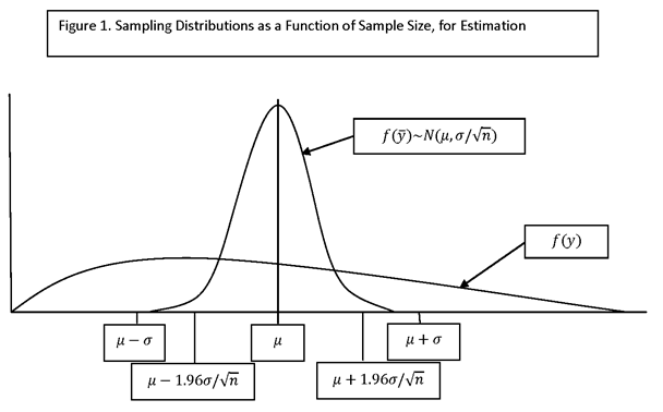
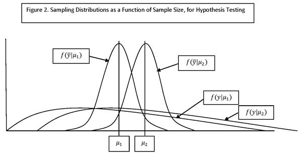
THE ISSUE OF SAMPLE SIZE DETERMINATION (OR ESTIMATION): WHAT SAMPLE SIZE IS REQUIRED TO ACHIEVE THE DESIRED LEVEL OF PRECISION FOR ESTIMATES OF INTEREST, OR THE DESIRED LEVEL OF POWER (PROBABILITY) FOR DETECTING AN EFFECT OF SPECIFIED SIZE.

IN BOTH CASES, FOR MANY APPLICATIONS, THE ISSUE OF SAMPLE SIZE IS DETERMINED LARGELY BY THE BUDGET AVAILABLE FOR DATA COLLECTION (FIELD SURVEY OPERATIONS). A FIRST STEP IN SAMPLE SIZE ESTIMATION IS TO ESTIMATE THE PRECISION AND POWER ASSOCIATED WITH THE LIKELY BUDGET. IF THE LEVEL OF PRECISION IS INADEQUATE OR THE POWER TO DETECT EFFECTS OF ANTICIPATED SIZE IS TOO LOW, THERE IS NO POINT TO CONDUCTING THE SURVEY AS DESIGNED.

GENERAL APPROACH TO SAMPLE SIZE ESTIMATION: SET SAMPLE SIZE TO ACHIEVE A DESIRED GOAL

FOR ESTIMATION, DESIRE HIGH PRECISION OF CERTAIN ESTIMATES

FOR HYPOTHESIS TESTING, DESIRE HIGH POWER FOR CERTAIN TESTS OF HYPOTHESIS

SPECIFIC APPROACH:

· FOR ESTIMATION, DETERMINE THE SAMPLE SIZE REQUIRED TO OBTAIN A CONFIDENCE INTERVAL (OF SPECIFIED CONFIDENCE COEFFICIENT) OF A SPECIFIED WIDTH

· FOR HYPOTHESIS TESTING, DETERMINE THE SAMPLE SIZE REQUIRED TO DETECT A SPECIFIED EFFECT SIZE (CALLED THE MINIMUM DETECTABLE EFFECT) WITH A SPECIFIED POWER (PROBABILITY)

FOR PROGRAM MONITORING AND EVALUATION, DATA MAY BE COLLECTED, STORED AND PROCESSED IN VARIOUS WAYS:

· PROGRAM ADMINISTRATIVE RECORDS

· GOVERNMENT RECORDS

· CLIENT RECORDS (E.G., HOSPITALS, SCHOOLS, BUSINESSES, BANKS)

· MANAGEMENT INFORMATION SYSTEM (E.G., AN EDUCATION MANAGEMENT INFORMATION SYSTEM)

· COMMERCIAL DATA VENDORS (E.G., GEOGRAPHIC INFORMATION SYSTEMS)

· SAMPLE SURVEY

THIS PRESENTATION ADDRESSES DETERMINATION (OR ESTIMATION) OF SAMPLE SIZE FOR SAMPLE SURVEYS. SOME DATA, FOR USE IN DESIGN AND ANALYSIS, MAY BE OBTAINED FROM THE OTHER SOURCES LISTED ABOVE, BUT THE PRINCIPAL ITEMS OF INTEREST ARE OBTAINED FROM DATA COLLECTION INSTRUMENTS USED FOR A PROBABILITY SAMPLE SELECTED FROM A POPULATION OF INTEREST.

FOR BACKGROUND, A CURSORY KNOWLEDGE OF BASIC STATISTICS AND SAMPLE SURVEY DESIGN IS ASSUMED. THIS PRESENTATION DOES NOT DESCRIBE HOW TO SPECIFY SAMPLE DESIGN STRUCTURE, BUT SIMPLY HOW TO SPECIFY SAMPLE SIZE FOR CERTAIN BASIC SAMPLE DESIGNS. MANY DETAILED EXAMPLES ARE PRESENTED. TO KEEP THE EXAMPLES "SELF-CONTAINED," KEY POINTS WILL BE REPEATED; FOR THIS REASON THERE IS A CERTAIN LEVEL OF REDUNDANCY IN THE EXAMPLES.

FOR THE PRESENTATION, A "CLASSICAL" (FREQUENTIST, NON-BAYESIAN) APPROACH IS TAKEN. WHAT THIS MEANS IS THAT PRIOR INFORMATION ABOUT THE POPULATION (E.G., VARIANCES AND CORRELATIONS) IS USED TO ASSIST SURVEY DESIGN (E.G., SAMPLE SIZE DETERMINATION, CLUSTER SIZE SPECIFICATION, STRATUM ALLOCATIONS), BUT OTHERWISE THE POPULATION DISTRIBUTION IS UNSPECIFIED (NO PRIOR DISTRIBUTION FOR THE POPULATION; POPULATION PARAMETERS VIEWED AS FIXED, NOT RANDOM VARIABLES). FOR APPLICATIONS INVOLVING LARGE SAMPLES, EITHER APPROACH WOULD PRODUCE SIMILAR RECOMMENDATIONS FOR SAMPLE SIZE.

THE THREE MAIN CLASSES OF INVESTIGATION USING STATISTICAL METHODS ARE:

EXPERIMENTAL DESIGNS: STRUCTURED EXPERIMENTS BASED ON THE USE OF RANDOMIZATION TO SELECT EXPERIMENTAL UNITS AND ASSIGN TREATMENT LEVELS TO THEM. THE INVESTIGATOR CONTROLS THE SELECTION OF UNITS AND ASSIGNMENT OF TREATMENT. DESIGNED EXPERIMENT. RANDOMIZED CONTROLLED TRIAL.

QUASI-EXPERIMENTAL DESIGNS: INVESTIGATIONS WHICH POSSESS THE STRUCTURE OF AN EXPERIMENTAL DESIGN, BUT IN WHICH SOME ASPECT OF RANDOMIZATION IS LACKING. LACK OF RANDOMIZED ASSIGNMENT TO TREATMENT MAY BE ADDRESSED BY MATCHING.

OBSERVATIONAL STUDIES: STUDIES LACKING BOTH STRUCTURE AND RANDOMIZATION. ANALYSIS OF AVAILABLE DATA. NO EXPERIMENTAL CONTROL. MAY INVOLVE SAMPLING.

THE METHODS PRESENTED HERE MAY BE APPLIED TO ALL THREE TYPES OF INVESTIGATIONS.

HISTORICAL NOTE: STATISTICAL METHODS FOR DETERMINING SAMPLE SIZE HAVE BEEN AVAILABLE FOR AT LEAST A CENTURY. CURIOUSLY, THE METHOD OF STATISTICAL POWER ANALYSIS TO DETERMINE SAMPLE SIZE HAS NOT BEEN WIDELY USED IN EVALUATION, UNTIL RELATIVELY RECENTLY.

IN THE FIELD OF QUALITY CONTROL, THE USE OF OPERATING CHARACTERISTIC CURVES (“OC” CURVES), WHICH PLOT 1 – POWER VERSUS EFFECT SIZE FOR VARIOUS SAMPLE SIZES, WERE WIDELY USED IN THE 1940s AND 1950s IN THE FIELD OF STATISTICAL QUALITY CONTROL. IN THE FIELD OF EXPERIMENTAL DESIGN, POWER CALCULATIONS WERE ROUTINELY DONE, WITH EXTENSIVE POWER CURVES PRESENTED IN Biometrika Tables for Statisticians (Biometrika Trust, 1^st ed. 1954, 2^nd ed. 1958, 3^rd ed 1966) (VOLUME I FOR t-TESTS AND VOLUME II FOR F TESTS). IN HIS CLASSIC TEXT, Testing Statistical Hypotheses (2^nd ed., Wiley, 1986, 1^st ed. 1959), E. L. LEHMANN OBSERVES, “THERE IS LITTLE POINT IN CARRYING OUT AN EXPERIMENT WHICH HAS ONLY A SMALL CHANCE OF DETECTING THE EFFECT BEING SOUGHT WHEN IT EXISTS. SURVEYS BY COHEN (1962) AND FREIMAN ET AL. (1978) SUGGEST THAT THIS IS IN FACT THE CASE FOR TOO MANY STUDIES. IDEALLY, THE SAMPLE SIZE SHOULD THEN BE INCREASED TO PERMIT ADEQUATE VALUES FOR BOTH SIGNIFICANCE AND POWER.”

MANY TEXT AND REFERENCE BOOKS ON SAMPLE SURVEY CONSIDER ONLY DESCRIPTIVE SURVEYS, AND DO NOT ADDRESS, OR EVEN MENTION, STATISTICAL POWER ANALYSIS TO DETERMINE SAMPLE SIZE FOR ANALYTICAL SURVEYS.

REFERENCES ON SAMPLE SIZE DETERMINATION:

DESCRIPTIVE SURVEYS (PRECISION ANALYSIS)

Lohr, Sharon L., Sampling: Design and Analysis, 2nd ed., Cengage Learning, 2009

Scheaffer, Richard L, William Mendenhall and Lyman Ott, Elementary Survey Sampling, 2^nd ed, Duxbury Press, 1979

Thompson, Steven K., Sampling, 3^rd ed., Wiley, 2012

ANALYTICAL SURVEYS (STATISTICAL POWER ANALYSIS)

Cohen, Jacob, Statistical Power Analysis for the Behavioral Sciences, 2^nd ed., Lawrence Erlbaum Associates, 1988 (1^st ed. Academic Press, 1969)

Bloom, Howard S., ed., Learning More from Social Experiments: Evolving Analytic Approaches, an MDRC Project, Russell Sage Foundation, 2005.

TREATMENT OF NONRESPONSE AND NONCOMPLIANCE

THE FORMULAS AND EXAMPLES TO BE PRESENTED DO NOT TAKE INTO ACCOUNT NONRESPONSE, WHICH CAN OCCUR FOR MANY REASONS. FOR MULTISTAGE SURVEYS, THE NONRESPONSE RATE WILL DIFFER FOR SAMPLE UNITS AT DIFFERENT LEVELS. THE SURVEY INSTRUMENTS AND PROTOCOL MAY INCLUDE PROVISIONS FOR NONRESPONSE, SUCH AS COLLECTING DATA THAT MAY BE RELATED TO NONRESPONSE, SUCH AS THE CALL-BACK NUMBER ON WHICH A RESPONSE WAS OBTAINED. PROVISION FOR NONRESPONSE IN LONGITUDINAL SURVEYS (USUALLY CALLED ATTRITION) SHOULD TAKE INTO ACCOUNT THE NUMBER AND TIMING OF SURVEY ROUNDS.

NONRESPONSE IN LONGITUDINAL SURVEYS IN WHICH THE SAME UNITS (E.G., HOUSEHOLDS) ARE INTERVIEWED IN SUCCESSIVE SURVEY ROUNDS (PANEL SURVEYS) CAN HAVE A VERY DELETERIOUS EFFECT ON THE PRECISION OF “DIFFERENCE” ESTIMATES, AND THERE IS NOT MUCH THAT CAN BE DONE ABOUT IT APART FROM INCREASING THE SAMPLE SIZE IN THE INITIAL (BASELINE) SURVEY. NONRESPONSE OF UNITS THAT RESPONDED IN A PRIOR SURVEY ROUND IS CALLED “ATTRITION.”

NONRESPONSE AFFECTS THE ACCURACY OF SURVEY ESTIMATES WITH RESPECT TO BOTH PRECISION AND BIAS. WITH RESPECT TO PRECISION, MANY SURVEYS ALLOW FOR REPLACEMENT OF NONRESPONDENTS, SUCH AS REPLACING A NONRESPONDING HOUSEHOLD IN A VILLAGE BY ANOTHER HOUSEHOLD IN THE VILLAGE. THIS APPROACH MAINTAINS PRECISION AND FACILITATES CONTRACTING FOR FIELD WORK (WHEN CONTRACTS ARE SET UP FOR PAYMENT ACCORDING TO THE NUMBER OF COMPLETED INTERVIEWS). USUALLY, NONRESPONSE IS LOW FOR HIGHER LEVELS OF SAMPLING, E.G., IT IS UNLIKELY THAT A DISTRICT OR VILLAGE WILL BE NONRESPONDING.

IN ORDER TO KEEP NONRESPONSE BIAS LOW, THE PROTOCOL FOR MAKING REPLACEMENTS SHOULD ASSURE THAT THEY ARE AS SIMILAR AS POSSIBLE TO THE NONRESPONDING UNITS, WITH RESPECT TO VARIABLES THAT MAY AFFECT OUTCOMES OF INTEREST. (FOR EXAMPLE, REPLACE A NONRESPONDING HOUSEHOLD BY A SIMILAR ONE IN THE SAME VILLAGE.)

AS A GENERAL RULE, TO ACCOUNT FOR NONRESPONSE, INCREASE THE SAMPLE SIZE AT EACH LEVEL OF SAMPLING BY AN AMOUNT SUFFICIENT TO ASSURE THAT THE FINAL SAMPLE SIZE WILL LIKELY EQUAL OR EXCEED THE SAMPLE SIZE REQUIRED TO ACHIEVE A SPECIFIED LEVEL OF PRECISION OR POWER ASSUMING NO NONRESPONSE.

NONRESPONSE WILL BE MENTIONED IN SOME OF THE EXAMPLES PRESENTED, BUT IN MOST INSTANCES THE EXAMPLES WILL PRESENT SAMPLE SIZE ESTIMATES INDEPENDENTLY OF NONRESPONSE.

“NONCOMPLIANCE” REFERS TO THE FACT THAT SUBJECTS MAY NOT COMPLY WITH THE EXPERIMENTAL PROTOCOL; FOR EXAMPLE, CONTROL UNITS MAY BECOME TREATMENT UNITS. THE OCCURRENCE OF NONCOMPLIANCE CHANGES THE SAMPLE SIZES FOR THE TREATMENT AND CONTROL GROUPS. NONCOMPLIANCE IS NOT TAKEN INTO ACCOUNT IN THE DISCUSSION THAT FOLLOWS. TO THE EXTENT THAT IT IS ANTICIPATED, SAMPLE-SIZE ESTIMATES SHOULD BE INCREASED AS APPROPRIATE.

2. SAMPLE SURVEYS FOR MONITORING AND EVALUATION -OVERVIEW

DESCRIPTIVE SURVEYS (FOR MONITORING)

· ESTIMATE OVERALL CHARACTERISTICS OF A PARTICULAR, FIXED, FINITE POPULATION OR SUBPOPULATIONS OF INTEREST.

· “DESIGN-BASED” APPROACH AND ESTIMATES: UNDER THIS “FIXED POPULATION” APPROACH, NO STOCHASTIC MODEL IS SPECIFIED FOR THE VALUES OF THE POPULATION UNITS. A STOCHASTIC MODEL IS SPECIFIED FOR THE SAMPLE SELECTION (SAMPLE DESIGN AND SAMPLE SELECTION PROCEDURE).

· IT IS OFTEN ASSUMED THAT THE MODEL DESIGN PARAMETERS ARE “FIXED EFFECTS,” NOT RANDOM EFFECTS.

ANALYTICAL SURVEYS (FOR EVALUATION)

· ESTIMATE THE IMPACT (EFFECT) OF A PROGRAM INTERVENTION, OR THE RELATIONSHIP OF IMPACT TO EXPLANATORY VARIABLES

· “MODEL-BASED” APPROACH AND ESTIMATES: CAUSAL MODELING. UNDER THIS “STOCHASTIC POPULATION” APPROACH, THE POPULATION OF INTEREST IS A CONCEPTUALLY INFINITE SET OF POPULATIONS FROM WHICH THE SURVEYED POPULATION IS CONSIDERED TO BE A PARTICULAR REALIZATION, OR SAMPLE. THE POPULATION WOULD BE DIFFERENT IF THE PROGRAM INTERVENTION WERE VARIED. A STOCHASTIC MODEL IS SPECIFIED FOR THE RELATIONSHIP OF OUTCOMES OF INTEREST TO EXPLANATORY VARIABLES OF INTEREST (E.G., RESPONSE TO TREATMENT).

· MAY ALSO CONSIDER “MODEL-ASSISTED” APPROACH, WHICH INCLUDES BOTH A CAUSAL MODEL AND THE SAMPLE DESIGN. IF MODEL IS WELL SPECIFIED IN TERMS OF EXPLANATORY VARIABLES, DON’T NEED TO INCLUDE DESIGN IN MODEL. PERFORM ESTIMATION WITH AND WITHOUT SAMPLE “WEIGHTS.” THIS DISTINCTION IS NOT RELEVANT TO SAMPLE SIZE ESTIMATION.

· MOST EXPLANATORY VARIABLES ARE ASSUMED TO BE “RANDOM EFFECTS,” NOT FIXED EFFECTS. SOME OF THE DESIGN VARIABLES ARE FIXED EFFECTS (E.G., SURVEY ROUND, TREATMENT EFFECTS, SOME VARIABLES OF STRATIFICATION), AND OTHERS ARE ASSUMED TO BE RANDOM EFFECTS (E.G., THE CLUSTERS IN CLUSTER SAMPLING, COVARIATES). WHETHER AN EFFECT IS ASSUMED TO BE FIXED OR RANDOM MAY MAKE A VERY LARGE DIFFERENCE IN SAMPLE-SIZE REQUIREMENTS.

THE SAMPLE SIZE ESTIMATES MAY VARY SUBSTANTIALLY, DEPENDING ON WHETHER THE SURVEY IS DESCRIPTIVE OR ANALYTICAL.

NOTE ON TERMINOLOGY: THE TERM “MODEL-BASED” IS A LITTLE AMBIGUOUS. A “DESIGN-BASED” ESTIMATE IS IN FACT BASED ON A STATISTICAL MODEL. MORE PRECISE TERMINOLOGY WOULD BE “DESIGN-MODEL-BASED” (INSTEAD OF “DESIGN-BASED”) AND “CAUSAL-MODEL-BASED” (INSTEAD OF “MODEL-BASED”) .

3. SAMPLE SIZE ESTIMATION FOR DESCRIPTIVE SURVEYS

SAMPLE SIZE DEPENDS ON:

· THE ESTIMATOR OF INTEREST (E.G., A MEAN, PROPORTION OR TOTAL)

· THE LEVEL OF PRECISION DESIRED (E.G., WIDTH OF A 95% CONFIDENCE INTERVAL FOR A POPULATION MEAN; “ERROR BOUND”)

· POPULATION CHARACTERISTICS (STANDARD DEVIATIONS, INTERNAL HOMOGENEITY OF POTENTIAL SAMPLING UNITS (E.G., VILLAGES) OR STRATA, SUBPOPULATIONS OF INTEREST)

· SURVEY COSTS (E.G., RELATIVE COST OF SAMPLING A VILLAGE VS. SAMPLING A HOUSEHOLD)

· SURVEY DESIGN (E.G., WHETHER TO USE SIMPLE RANDOM SAMPLING, CLUSTER SAMPLING, MULTISTAGE SAMPLING OR STRATIFIED SAMPLING)

SOME OBSERVATIONS:

THE ONLY RANDOM VARIABLE CONSIDERED HERE IS THE SELECTION EVENT (OF INCLUSION IN THE SAMPLE). THE POPULATION IS CONSIDERED FIXED.

THE TOPIC OF SAMPLE SURVEY DESIGN IS BROAD, AND SOME GENERAL KNOWLEDGE OF THAT FIELD IS ASSUMED HERE. REFERENCES (DESCRIPTIVE SAMPLE SURVEY DESIGN):

· Lohr, Sharon L., Sampling: Design and Analysis, 2nd ed., Cengage Learning, 2009

· Scheaffer, Richard L, William Mendenhall, R. Lyman Ott and Kenneth G. Gerow, Elementary Survey Sampling, 7th ed., Cengage Learning, 2011

· Cochran, William G., Sampling Techniques, 3^rd ed., Wiley, 1977

MAJOR TYPES OF SAMPLE SURVEY DESIGNS

· SIMPLE RANDOM SAMPLING (srs)

· SINGLE-STAGE CLUSTER SAMPLING (clus)

· MULTISTAGE SAMPLING (multi)

· STRATIFIED SAMPLING (strat)

SAMPLE SIZE ESTIMATION IS DONE AT DIFFERENT STAGES OF A STUDY, TAKING INTO ACCOUNT THE INFORMATION THAT IS AVAILABLE AT THE TIME:

· PRELIMINARY ESTIMATES (E.G., FOR A PROPOSAL)

· FINAL ESTIMATES (SAMPLE DESIGN TASK)

USUALLY, NOT ALL OF THE DATA REQUIRED TO CONSTRUCT AN ACCURATE ESTIMATE OF SAMPLE SIZE IS AVAILABLE, AND THE ESTIMATE IS BASED ON A NUMBER OF ASSUMPTIONS. IT IS USEFUL TO CONDUCT A “SENSITIVITY ANALYSIS” TO SHOW THE DEPENDENCE OF THE SAMPLE SIZE ESTIMATE ON THE ASSUMPTIONS MADE.

THE APPROACH HERE WILL BE TO CONSTRUCT SAMPLE-SIZE ESTIMATES FOR A NUMBER OF BASIC SAMPLE-SURVEY DESIGNS (I.E., THOSE LISTED ABOVE). THE DESIGNS USED WILL BE DESCRIBED BY MODELS INVOLVING JUST A FEW DESIGN PARAMETERS THAT ARE RELATIVELY EASY TO ESTIMATE. IT IS NOT USEFUL TO SPECIFY A COMPLEX DESIGN MODEL WITH MANY PARAMETERS WHOSE VALUES ARE NOT KNOWN OR READILY SPECIFIED PRIOR TO OBTAINING THE SURVEY DATA, OR THAT DO NOT AFFECT PRECISION MUCH. SAMPLE SIZE WILL BE ESTIMATED BASED ON REASONABLE VALUES FOR A SMALL NUMBER OF IMPORTANT DESIGN PARAMETERS.

THE INTENDED APPLICATION FOR THE RESULTS PRESENTED HERE IS A REQUIREMENT TO PRODUCE A PRELIMINARY ESTIMATE OF SAMPLE SIZE, BASED ON GENERAL CHARACTERISTICS OF THE POPULATION AND PLANNED SURVEY. IT IS NOT INTENDED TO CONSTRUCT A FINAL DESIGN OR SAMPLE SIZE, WHICH MAY DEPEND ON ADDITIONAL DATA AND MORE ELABORATE MODELS.

THE MODELS ON WHICH SAMPLE SIZE ESTIMATES ARE BASED WILL BE SIMPLE, BUT NOT OVERLY SIMPLE. THE MODEL MUST BE AN ADEQUATE APPROXIMATION OF REALITY. A STRATIFIED DESIGN, FOR EXAMPLE, COULD BE MUCH MORE PRECISE OR MUCH LESS PRECISE FOR CERTAIN ESTIMATES THAN A SIMPLE RANDOM SAMPLE, DEPENDING ON THE POPULATION CHARACTERISTICS AND ALLOCATION OF THE SAMPLE TO THE STRATA.

KEY ASSUMPTIONS:

LARGE SAMPLE SIZE: IT IS ASSUMED THAT THE SAMPLE SIZES ARE LARGE (E.G., SEVERAL HUNDRED HOUSEHOLD INTERVIEWS CONDUCTED IN 30 SAMPLE VILLAGES). THIS ASSUMPTION IS NOT ESSENTIAL BUT IT SIMPLIFIES THE FORMULAS, AND THIS PRESENTATION.

BINARY TREATMENT: FOR MOST OF THE DISCUSSION, IT IS ASSUMED THAT THERE ARE TWO LEVELS OF TREATMENT: TREATED AND UNTREATED (OR COMPARISON OR CONTROL). (THE TERM “CONTROL” IS USUALLY RESERVED FOR USE WITH EXPERIMENTAL DESIGNS, IN WHICH TREATMENT IS ASSIGNED BY RANDOMIZATION, AND “COMPARISON” FOR QUASI-EXPERIMENTAL DESIGNS OR OBSERVATIONAL STUDIES.) SOME MATERIAL WILL BE PRESENTED ABOUT MULTIPLE TREATMENT LEVELS AND MULTIVARIATE OUTCOMES (MULTIPLE OUTCOME VARIABLES OF INTEREST).

ADJUSTMENT FOR COVARIATES: IN MANY APPLICATIONS, PRELIMINARY SAMPLE-SIZE ESTIMATES DO NOT TAKE INTO ACCOUNT ESTIMATES THAT ADJUST FOR COVARIATES. THIS IS A CONSERVATIVE APPROACH (SINCE ADJUSTMENT FOR COVARIATES USUALLY INCREASES POWER AND ALLOWS FOR SMALLER SAMPLE SIZES). FOR DOUBLE-DIFFERENCE ESTIMATORS, ADJUSTMENT FOR COVARIATES OFTEN MAKES LITTLE DIFFERENCE IN POWER. MOST OF THE DISCUSSION HERE ASSUMES NO ADJUSTMENT FOR COVARIATES. THAT TOPIC IS ADDRESSED BRIEFLY, IN A FEW SPECIAL CASES. IT IS OF GREATER INTEREST IN ESTIMATING SAMPLE SIZE IN CONSTRUCTING DETAILED DESIGN, NOT IN PRELIMINARY ESTIMATION OF SAMPLE SIZE. TO BE USEFUL, MUCH ADDITIONAL INFORMATION ABOUT THE POPULATION IS REQUIRED (E.G., FROM SIMILAR PREVIOUS SURVEYS).

NOTE: THE OPTIMAL SURVEY DESIGN VARIES BY THE ESTIMATES OF INTEREST, SINCE THE STOCHASTIC PROPERTIES THAT AFFECT SAMPLE SIZE (E.G., STANDARD DEVIATIONS, INTRA-CLUSTER CORRELATION COEFFICIENTS) MAY DIFFER FOR EACH VARIABLE. HENCE, SAMPLE SIZE IS USUALLY ESTIMATED FOR A RANGE OF VALUES OF IMPORTANT PARAMETERS (“SENSITIVITY ANALYSIS”) FOR IMPORTANT OUTCOMES OF INTEREST.

SURVEY DESIGNS TO BE CONSIDERED:

· SIMPLE RANDOM SAMPLING

· SINGLE-STAGE CLUSTER SAMPLING

· TWO-STAGE SAMPLING (CLUSTER SAMPLING WITH SUBSAMPLING)

· STRATIFIED SAMPLING

IN ADDITION, THE PRECEDING DESIGNS WILL BE CONSIDERED IN THE FOLLOWING SITUATIONS:

· SINGLE ROUND (TIME) OF SAMPLING, NO SUBPOPULATIONS OF INTEREST

· SINGLE ROUND OF SAMPLING, SUBPOPULATIONS (E.G., TREATED VS. UNTREATED, MALES VS FEMALES, REGIONS, TREATMENT MODALITIES)

· TWO ROUNDS OF SAMPLING

QUANTITIES TO BE ESTIMATED (PARAMETER, ESTIMAND, MEASURE OF INTEREST):

· POPULATION CHARACTERISTICS SUCH AS MEANS, PROPORTIONS AND TOTALS OF THE ENTIRE POPULATION AND SUBPOPULATIONS

· VARIOUS MEASURES OF INTEREST, SUCH AS MEASURES OF IMPACT OF A PROGRAM INTERVENTION

o SINGLE DIFFERENCE IN GROUP MEANS

o DOUBLE DIFFERENCE IN GROUP MEANS

· RELATIONSHIPS, SUCH AS RATIOS AND REGRESSION ESTIMATES

ESTIMATION OF TOTALS IS SIMILAR TO ESTIMATION OF MEANS, AND WILL NOT BE DISCUSSED SEPARATELY.

GENERAL APPROACH TO SAMPLE SIZE ESTIMATION FOR DESCRIPTIVE SURVEYS

FOR A MEASURE OF INTEREST (SUCH AS A POPULATION MEAN), DETERMINE A CONFIDENCE INTERVAL FOR WHICH THE WIDTH, +E OR 2E, IS A KNOWN FUNCTION OF SAMPLE SIZE, n. SET THE WIDTH OF THE CONFIDENCE INTERVAL AND SOLVE FOR n. THE HALF-WIDTH, E, IS CALLED THE “ERROR BOUND.”

IN THE FOLLOWING, THE CONFIDENCE INTERVAL (AN “INTERVAL ESTIMATE”) WILL BE BASED ON A POINT ESTIMATE, AND THE SAMPLING DISTRIBUTION OF THE POINT ESTIMATE WILL BE APPROXIMATED BY APPLYING “LARGE-SAMPLE” (OR “ASYMPTOTIC”) THEORY (I.E., BY INVOKING THE LAW OF LARGE NUMBERS AND THE CENTRAL LIMIT THEOREM (IN PARTICULAR, HÁJEK’S VERSION, FOR SIMPLE RANDOM SAMPLING WITHOUT REPLACEMENT)). A NUMBER OF SPECIFIC CASES WILL BE CONSIDERED, STARTING WITH ESTIMATION OF THE POPULATION MEAN USING THE SAMPLE MEAN FROM A SIMPLE RANDOM SAMPLE, AND THEN MOVING TO MORE COMPLEX DESIGNS AND MEASURES.

LET M DENOTE A MEASURE OF INTEREST (SUCH AS A POPULATION MEAN). LET m DENOTE AN ESTIMATOR OF M FOR WHICH THE LAW OF LARGE NUMBERS AND THE CENTRAL LIMIT THEOREM APPLY (I.E., THE ESTIMATOR CONVERGES TO M AS THE SAMPLE SIZE INCREASES, AND THE SAMPLING DISTRIBUTION OF THE ESTIMATOR IS APPROXIMATELY NORMAL). THESE CONDITIONS WILL APPLY IN ALL OF THE CASES CONSIDERED HERE. DENOTE THE VARIANCE OF m BY σ²_m, AND THE STANDARD DEVIATION (OR STANDARD ERROR) OF m BY σ_m.

THEN, UNDER THE ASSUMPTIONS MADE, FOR LARGE SAMPLES m IS APPROXIMATELY NORMALLY DISTRIBUTED WITH MEAN M AND VARIANCE σ_m, AND SO THE APPROXIMATE DISTRIBUTION OF THE QUANTITY

IS A STANDARD NORMAL DISTRIBUTION. HENCE

WHERE

c = confidence coefficient (e.g., .95)

z_γ = 1 – γ percentile of the standard normal distribution (i.e., the standard normal deviate having probability γ to the right (e.g., for c = .95, (1-c)/2 = .025, in which case z_.025 = 1.96)

REARRANGING:

HENCE THE INTERVAL

IS A 100c PERCENT CONFIDENCE INTERVAL FOR M.

NOTATION: THE SUBSCRIPT (1 – c)/2 OCCURS A LOT IN THE PRESENTATION THAT FOLLOWS. TO SIMPLIFY THE FORMULAS, IT IS CUSTOMARY TO WRITE THE CONFIDENCE COEFFICIENT c AS c = 1 – α, IN WHICH CASE (1-c)/2 = α/2. (THE PARAMETER α DOES NOT HAVE A NAME.)

USING THIS NOTATION, THE PRECEDING CONFIDENCE INTERVAL BECOMES

IN THE CASES WE WILL CONSIDER, THE STANDARD DEVIATION, σ_m, IS A DECREASING FUNCTION OF n, THE SAMPLE SIZE. THE VALUE OF n IS DETERMINED SO THAT THE CONFIDENCE INTERVAL IS OF THE DESIRED WIDTH.

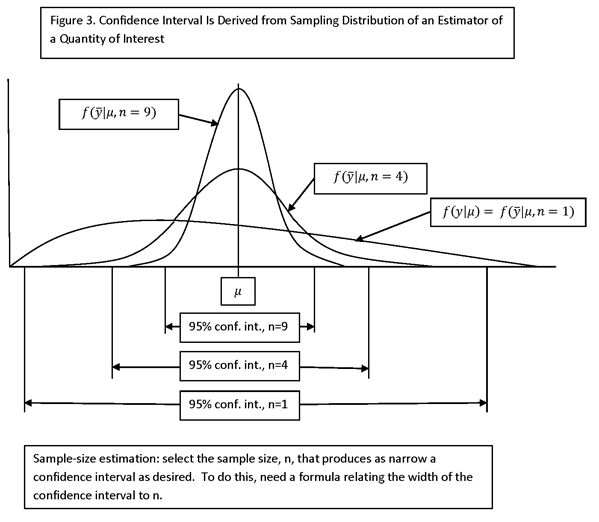
THE APPROACH TO ESTIMATING SAMPLE SIZE DEPENDS ON KNOWING A FORMULA FOR THE VARIANCE OF THE POINT ESTIMATE, m, THAT DEPENDS ON THE SAMPLE SIZE, n. TO KEEP THE FORMULAS SIMPLE, SPECIAL CASES ARE EXAMINED, SUCH AS “BALANCED” DESIGNS, AND A NUMBER OF APPROXIMATIONS ARE MADE. IN MANY SAMPLE-SIZE-ESTIMATION PROBLEMS, NOT A LOT IS KNOWN ABOUT THE POPULATION PRIOR TO THE SURVEY (APART FROM A FRAME FOR SAMPLING), AND THERE IS NO POINT TO SPECIFYING HIGHLY COMPLEX DESIGNS FOR WHICH THE PARAMETERS ARE NOT KNOWN).

NOTE: IN MUCH OF THE DISCUSSION THAT FOLLOWS, IT WILL BE ASSUMED THAT THE POPULATION SIZE, N, IS LARGE COMPARED TO THE SAMPLE SIZE, n. THIS IS DONE TO SIMPLIFY THE PRESENTATION (THE FORMULAS FOR STANDARD ERRORS ARE SIMPLER). IF THIS CONDITION DOES NOT APPLY, AND THE SAMPLE IS AN APPRECIABLE PORTION OF THE POPULATION, THE VARIANCE OF SAMPLE ESTIMATES MAY BE REDUCED (AND SAMPLE-SIZE ESTIMATES REDUCED) BY USING SAMPLING WITHOUT REPLACEMENT.

FOR SIMPLE RANDOM SAMPLING WITHOUT REPLACEMENT, THE VARIANCE IS REDUCED BY THE FACTOR 1 – n/N, WHICH IS CALLED THE FINITE POPULATION CORRECTION, OR fpc. IN MULTISTAGE SAMPLING, SUCH FACTORS APPLY TO EACH LEVEL OF SAMPLING. CLEARLY, IF THE SAMPLE IS AN APPRECIABLE PORTION OF THE POPULATION, THE REDUCTION IN VARIANCES BY USING NONREPLACEMENT SAMPLING IS SUBSTANTIAL.

NOTE: FORMULAS INVOLVING N AND THE fpc DIFFER, DEPENDING ON WHETHER THE VARIANCE OF A FINITE POPULATION IS DEFINED AS OR . WHILE THE FIRST DEFINITION IS MORE NATURAL (AND UNBIASED), THE SECOND DEFINITION RESULTS IN SIMPLER FORMULAS, AND WILL BE USED HERE.

AFTER DISCUSSING THIS SPECIAL CASE (N LARGE COMPARED TO n) IN DETAIL, RESULTS WILL BE PRESENTED FOR THE GENERAL CASE.

NOTE THAT “N LARGE COMPARED TO n” DOES NOT IMPLY THAT n IS SMALL. n MUST BE SUFFICIENTLY LARGE TO JUSTIFY APPLICATION OF THE LAW OF LARGE NUMBERS AND THE CENTRAL LIMIT THEOREM.

THE METHODOLOGY FOR SMALL n REQUIRES ASSUMPTIONS ABOUT THE DISTRIBUTION OF THE UNDERLYING RANDOM VARIABLE, THE RESPONSE Y. IF Y IS NORMALLY DISTRIBUTED, THEN THE DISTRIBUTION OF THE SAMPLE MEAN DIVIDED BY ITS ESTIMATED STANDARD ERROR IS A Student’s t DISTRIBUTION. THE FORMULAS FOR ESTIMATING SAMPLE SIZE IN THIS CASE ARE EXACTLY AS PRESENTED HERE, EXCEPT THAT THE PERCENTILE z_α/2 OF THE STANDARD NORMAL DISTRIBUTION IS REPLACED BY THE PERCENTILE t_α/2(df) OF A Student’s t DISTRIBUTION, WHERE df DENOTES THE NUMBER OF DEGREES OF FREEDOM. USING THE Student’s t DISTRIBUTION WILL RESULT IN SOMEWHAT WIDER CONFIDENCE INTERVALS. (THE DIFFERENCE IS SMALL WHEN n IS QUITE SMALL, SAY, LESS THAN 30. FOR n SUFFICIENTLY LARGE TO JUSTIFY INVOKING THE LAW OF LARGE NUMBERS OR THE CENTRAL LIMIT THEOREM, THE APPROXIMATION IS QUITE APPROPRIATE.)

THE METHODOLOGY FOR MULTIPLE TREATMENT LEVELS VARIES, DEPENDING ON WHETHER THE TREATMENT LEVELS ARE CATEGORICAL OR CONTINUOUS. IF CATEGORICAL, THE USUAL GOAL IS TO TEST THE HYPOTHESIS OF EQUALITY OF TREATMENTS (ADDRESSED IN THE NEXT SECTION). IF CONTINUOUS, THE GOAL MAY BE TO ESTIMATE A MINIMUM LETHAL DOSE, OR TO ESTIMATE THE RELATIONSHIP OF OUTCOME TO AN EXPLANATORY VARIABLE.

CASE 1: SIMPLE RANDOM SAMPLING, ESTIMATION OF THE POPULATION MEAN, μ, FROM A SAMPLE, y₁, y₂,…,y_n, USING THE SAMPLE MEAN, , AS THE ESTIMATOR FOR μ.

THIS TYPE OF DESIGN IS UNUSUAL, SINCE MORE EFFICIENT DESIGNS CAN USUALLY BE FOUND. IT IS MOST USEFUL AS A COMPARISON, WHEN CONSIDERING THE PRECISION OF OTHER, MORE COMPLEX, DESIGNS.

GIVEN: RESPONSE (OUTCOME) VARIABLE Y FOR WHICH THE POPULATION MEAN IS μ AND POPULATION STANDARD DEVIATION IS σ.

BY THE LAW OF LARGE NUMBERS, FOR LARGE SAMPLES THE SAMPLE MEAN, , IS A CONSISTENT ESTIMATOR OF THE POPULATION MEAN, μ.

BY THE CENTRAL LIMIT THEOREM, THE SAMPLE MEAN IS APPROXIMATELY NORMALLY DISTRIBUTED WITH MEAN μ AND VARIANCE σ²/n.

HENCE THE FOLLOWING APPROXIMATION HOLDS:

where

= standard deviation of

c = confidence coefficient (e.g., .95)

α = 1 - c

z_γ = standard normal deviate having probability γ to the left (e.g., for γ = .025, z_.025 = -1.96 and z_.975 = 1.96)

REFER TO FIGURE 3.

REARRANGING:

HENCE THE INTERVAL

IS A 100c PERCENT CONFIDENCE INTERVAL FOR μ.

NOTE: FOR DESCRIPTIVE SURVEYS, μ IS NOT CONSIDERED TO BE A RANDOM VARIABLE (IN THIS “CLASSICAL,” NON-BAYESIAN APPROACH). THE CONFIDENCE INTERVAL, AN INTERVAL ESTIMATE, IS A RANDOM VARIABLE. THE INTERPRETATION IS THAT IF WE ADOPT THIS APPROACH TO INFERENCE, THE CONFIDENCE INTERVAL WILL INCLUDE THE TRUE VALUE, μ, IN 100c PERCENT OF THE APPLICATIONS.

IF WE DESIRE THAT THE HALF-WIDTH OF THE CONFIDENCE INTERVAL BE E, THEN

SOLVING FOR n WE OBTAIN

NOTE THAT FOR c = .95, z_α/2 IS 1.96, OR APPROXIMATELY 2, IN WHICH CASE n IS APPROXIMATELY EQUAL TO 4σ²/E².

THE VALUE c = .95 (α = .05) IS THE MOST COMMONLY USED VALUE FOR THE CONFIDENCE COEFFICIENT, CORRESPONDING TO z = 1.96 (OFTEN ROUNDED TO 2). OTHER VALUES ARE c = .90 AND c = .99, FOR WHICH THE VALUES OF z ARE 1.645 AND 2.50.

THE PRECEDING DISCUSSION ASSUMED THAT THE POPULATION SIZE, N, IS LARGE COMPARED TO THE SAMPLE SIZE, n. IF THIS IS NOT THE CASE, THE VARIANCE OF IS REDUCED BY THE fpc, AND THE FORMULA FOR ESTIMATING THE SAMPLE SIZE BECOMES:

OR, FOR A 95% CONFIDENCE INTERVAL OF SIZE +E, APPROXIMATELY

EXAMPLE

PROBLEM STATEMENT:

SIMPLE RANDOM SAMPLING WITHOUT REPLACEMENT FROM A POPULATION OF SIZE N = 1,000,000.

ESTIMATION OF THE POPULATION MEAN FOR A VARIABLE HAVING STANDARD DEVIATION σ = 100.

DETERMINE THE SAMPLE SIZE REQUIRED TO ESTIMATE THE POPULATION MEAN WITH AN ERROR BOUND OF +10.

SOLUTION:

WHEN, AS IS THE CASE HERE, THE CONFIDENCE COEFFICIENT IS NOT SPECIFIED, WE ASSUME IN THE FORMULA FOR n THAT = 4, CORRESPONDING TO AN APPROXIMATE 95% CONFIDENCE COEFFICIENT.

DETERMINE THE SAMPLE SIZE REQUIRED TO OBTAIN A 95% CONFIDENCE INTERVAL FOR THE POPULATION MEAN OF SIZE +10.

THE FOLLOWING TABLE SOLVES THIS SAME (SECOND) PROBLEM FOR VARYING VALUES OF N, FOR BOTH SIMPLE RANDOM SAMPLING WITHOUT REPLACEMENT AND FOR SIMPLE RANDOM SAMPLING WITH REPLACEMENT. FOR N LARGE COMPARED TO n, THE POPULATION SIZE HAS LITTLE EFFECT ON THE REQUIRED SAMPLE SIZE, AND WHETHER SAMPLING IS WITH OR WITHOUT REPLACEMENT.

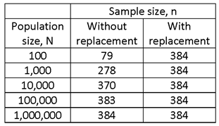
FOR SMALL POPULATIONS, THE FINITE POPULATION HAS A SUBSTANTIAL EFFECT, AND SO, IF SAMPLING WITH REPLACEMENT IS USED THE REQUIRED SAMPLE TO OBTAIN THE REQUIRED PRECISION IS MUCH SMALLER. FOR VERY SMALL POPULATIONS, SUCH AS N = 100, THE SAMPLE SIZE IS SUCH A LARGE PORTION OF THE POPULATION THAT THERE IS LITTLE POINT TO SAMPLING (I.E., MEASURE ALL OF THE UNITS OF THE POPULATION).

MANY PEOPLE FIND IT COUNTER-INTUITIVE THAT THE SAMPLE SIZE REQUIRED TO OBTAIN A CERTAIN LEVEL OF PRECISION DOES NOT INCREASE WITH POPULATION SIZE, EXCEPT FOR SMALL POPULATIONS.

SAMPLING FOR PROPORTIONS

IN THE CASE IN WHICH THE RESPONSE VARIABLE Y IS A BINARY EVENT (E.G., “NO” OR “YES”, DENOTED BY 0 OR 1), THE POPULATION MEAN μ AND SAMPLE MEAN ARE PROPORTIONS, DENOTED BY p AND .

IN THIS CASE, THE STANDARD DEVIATION OF X IS . THE MAXIMUM VALUE OF σ IN THIS CASE IS .5. FOR THIS VALUE, THE VALUE OF n IS

FOR c = .95, IS APPROXIMATELY EQUAL TO 4, AND THIS IS APPROXIMATELY n = 1/E².

EXAMPLE

THE SAMPLE SIZE REQUIRED TO PRODUCE AND ERROR BOUND OF +3% IN SAMPLING FOR PROPORTIONS FROM A LARGE POPULATION IS

n = .25(1.96)²/.03² = 1,067.

THE SAMPLE SIZE OF 1,000 IS OFTEN USED BY TELEVISION OPINION POLLS, AND THE ERROR BOUND IS STATED TO BE +3% .

A KEY POINT IN SAMPLING FOR PROPORTIONS IS THAT IF p IS SPECIFIED, THEN σ IS KNOWN (I.E., IS ). IN MANY APPLICATIONS, IT IS DIFFICULT TO OBTAIN INFORMATION ABOUT σ PRIOR TO THE SURVEY, FOR USE IN ESTIMATING SAMPLE SIZE. FURTHERMORE, THE VALUE OF σ VARIES BY VARIABLE OF INTEREST (Y). FOR THESE REASONS, IT IS USEFUL TO SOLVE SAMPLE-SIZE PROBLEMS BY SPECIFYING THE MINIMUM DETECTABLE EFFECT SIZE (E) RELATIVE TO THE STANDARD DEVIATION, I.E., AS E_rel = E/σ. THE QUANTITY E_rel IS THE RELATIVE MINIMUM DETECTABLE EFFECT SIZE (RELATIVE TO THE STANDARD DEVIATION).

DIVIDING THE NUMERATOR AND DENOMINATOR OF THE EXPRESSION FOR n BY σ² YIELDS

WHICH IS INDEPENDENT OF σ.

THERE ARE TWO SUBSTANTIAL ADVANTAGES TO WORKING WITH THE RELATIVE MINIMUM DETECTABLE EFFECT:

· IT IS NOT NECESSARY TO KNOW THE VALUE OF σ

· THE SAMPLE SIZE ESTIMATE APPLIES TO ALL VARIABLES HAVING THE SPECIFIED VALUE OF E_rel.

ANOTHER APPROACH THAT MAY BE USED TO AVOID SPECIFICATION OF AN EXACT VALUE FOR THE STANDARD DEVIATION IS TO SPECIFY BOTH THE STANDARD DEVIATION AND THE EFFECT SIZE RELATIVE TO THE MEAN. THE STANDARD DEVIATION DIVIDED BY THE MEAN IS CALLED THE RELATIVE STANDARD DEVIATION. THE MINIMUM DETECTABLE EFFECT SIZE DIVIDED BY THE MEAN IS CALLED THE RELATIVE MINIMUM DETECTABLE EFFECT SIZE (RELATIVE TO THE MEAN).

DIVIDING THE NUMERATOR AND DENOMINATOR OF THE EXPRESSION FOR n BY μ² YIELDS

THE ADVANTAGE OF THIS FORMULA IS THAT IN MANY CASES THE RATIO OF THE STANDARD DEVIATION TO THE MEAN IS KNOWN APPROXIMATELY, ALTHOUGH THE ABSOLUTE VALUE OF THE STANDARD DEVIATION MAY NOT BE KNOWN.

AN EXAMPLE OF THIS FORMULATION IS ESTIMATION OF INCOME IN DEVELOPING COUNTRIES, WHERE THE STANDARD DEVIATION OF INCOME OF RURAL POOR IN MANY CASES VARIES BETWEEN .5 AND 2 TIMES THE MEAN INCOME. IN THIS CASE, IF IT IS DESIRED, FOR EXAMPLE, TO SPECIFY A SAMPLE SIZE THAT WOULD PRODUCE A 95% CONFIDENCE INTERVAL, THE PRECEDING FORMULA COULD BE USED, SETTING THE VALUE OF σ/μ EQUAL TO .5, 1, AND 2, AND SPECIFYING A VALUE (OR SEVERAL VALUES) FOR E/μ.

SAMPLE SIZE FOR ESTIMATION OF THE MEAN, FOR OTHER SAMPLE DESIGNS

FOR EACH OF THE FOLLOWING CASES IN WHICH SAMPLE SIZE IS ESTIMATED FOR DESCRIPTIVE SURVEYS, IT WILL BE ASSUMED THAT THE SAMPLE SIZE IS LARGE, SO THAT THE CENTRAL LIMIT THEOREM MAY BE INVOKED AND THE FOLLOWING FORMULA MAY BE USED AS A BASIS FOR DETERMINING CONFIDENCE INTERVALS AND SAMPLE SIZES FOR ESTIMATION OF THE POPULATION MEAN:

FOR THE OTHER CASES TO BE CONSIDERED (E.G., ESTIMATION OF DIFFERENCES), THE ESTIMATOR WILL BE SIMILAR TO THE CASE OF A SAMPLE MEAN, SUCH AS A (SINGLE) DIFFERENCE IN GROUP MEANS, OR A DOUBLE DIFFERENCE IN GROUP MEANS.

TO USE THIS APPROACH, IT IS NECESSARY TO HAVE AN EXPRESSION FOR THAT DEPENDS ON n. THE EXPRESSION WILL VARY DEPENDING ON THE SAMPLE DESIGN USED. IF WE DENOTE THE STANDARD DEVIATION OF USING SIMPLE RANDOM SAMPLING WITH REPLACEMENT (srswr) AS

AND THE STANDARD DEVIATION OF FOR AN ARBITRARY DESIGN, “des”, AS , THEN WE DEFINE THE DESIGN EFFECT, deff, AS

WITH THE INTRODUCTION OF deff, ALL THAT IS NECESSARY TO APPLY THE PRECEDING METHODOLOGY TO ESTIMATE SAMPLE SIZE FOR AN ARBITRARY DESIGN IS TO SPECIFY THE DESIGN EFFECT, deff.

(NOTE: LESLIE KISH DEFINED deff USING SIMPLE RANDOM SAMPLING WITHOUT REPLACEMENT AS THE BASIS FOR COMPARISON (I.E., FOR THE DENOMINATOR OF THE deff):

FOR N LARGE COMPARED TO n, THE TWO DEFINITIONS PRODUCE ABOUT THE SAME RESULT. BOTH DEFINITIONS ARE IN USE. ALSO IN USE AS A “DESIGN EFFECT” IS deft (INTRODUCED BY JOHN TUKEY), WHICH IS DEFINED AS THE RATIO OF THE STANDARD ERROR (INSTEAD OF THE VARIANCE) FOR THE DESIGN TO THE STANDARD ERROR FOR SIMPLE RANDOM SAMPLING (USUALLY WITH REPLACEMENT). IF deff IS USED, THE SAMPLE SIZE REQUIRED FOR A COMPLEX SURVEY TO ACHIEVE THE SAME PRECISION AS A SIMPLE RANDOM SAMPLE OF SAMPLE SIZE n IS n. IF deft IS USED, THE REQUIRED SAMPLE SIZE IS n deft.)

MANY SAMPLE SURVEYS INVOLVE MULTISTAGE SAMPLING, WHICH IS USUALLY LESS PRECISE (FOR MOST VARIABLES OF INTEREST) THAN SIMPLE RANDOM SAMPLING (FOR THE SAME SAMPLE SIZE) AND THE VALUE OF deff IS OFTEN ABOUT 3. FOR STRATIFIED SAMPLING, THE VALUE OF deff MAY BE LESS THAN 1.

ANOTHER NAME FOR THE DESIGN EFFECT IS THE VARIANCE INFLATION FACTOR, OR vif. THAT TERMINOLOGY WAS INTRODUCED BY A. DONNER. WE SHALL USE THE TERM VARIANCE INFLATION FACTOR AND THE NAME vif LATER, IN A MORE GENERAL CONTEXT. FOR THE MODELS CONSIDERED IN THIS SECTION (ESTIMATION OF MEANS), vif = deff.

CASE 2: SINGLE-STAGE CLUSTER SAMPLING, ESTIMATION OF THE POPULATION MEAN, μ, USING THE SAMPLE MEAN, AS THE ESTIMATOR FOR μ.

(A SINGLE-STAGE CLUSTER SAMPLE IS A SIMPLE RANDOM SAMPLE IN WHICH THE SAMPLING UNIT IS A COLLECTION, OR “CLUSTER” OF ELEMENTS. CLUSTER SAMPLING IS USEFUL WHEN THE CLUSTERS ARE INTERNALLY HETEROGENEOUS, SINCE, IF THE UNITS WITHIN CLUSTERS ARE VERY SIMILAR, THERE IS NO ADVANTAGE TO MEASURING A LOT OF THEM (THAT IS, OF THE UNITS WITHIN CLUSTERS).)

LET

h = number of clusters selected in the simple random sample

H = total number of clusters in the population

n = total number of elements (subunits) in the sample

N = total number of elements in the population

m_i = number of elements in the i-th cluster (or “size” of the i-th cluster)

y_i = total of the responses for all observations in the i-th cluster.

THEN THE SAMPLE MEAN IS GIVEN BY

NOTE THAT THE SAMPLE SIZE IN TERMS OF CLUSTERS IS h, BUT THE SAMPLE SIZE IN TERMS OF ELEMENTS (SUBUNITS, ULTIMATE SAMPLE UNIT) IS .

THE NOTATION USED HERE DIFFERS FROM SOME STANDARD SOURCES, WHICH USE n (INSTEAD OF h) TO DENOTE THE NUMBER OF CLUSTERS IN THE SAMPLE, AND N (INSTEAD OF H) TO DENOTE THE NUMBER OF CLUSTERS IN THE POPULATION. THE USE OF n TO DENOTE THE NUMBER OF ELEMENTS FOR SIMPLE RANDOM SAMPLING AND TO DENOTE THE NUMBER OF FIRST-STAGE UNITS FOR TWO-STAGE SAMPLING COMPLICATES THE DISCUSSION OF THE FORMULAS. THIS PRESENTATION WILL USE n THROUGHOUT TO REFER TO THE ELEMENT SAMPLE SIZE, AND N TO REFER TO THE ELEMENT POPULATION SIZE.

IF σ_w² DENOTES THE VARIANCE OF THE ELEMENTS WITHIN CLUSTERS AND σ_b² DENOTES THE VARIANCE OF THE CLUSTER MEANS, THEN THE QUANTITY ρ DEFINED BY

CALLED THE INTRA-CLUSTER CORRELATION COEFFICIENT, IS A MEASURE OF THE INTERNAL HOMOGENEITY OF CLUSTERS, I.E., OF THE EXTENT TO WHICH ELEMENTS WITHIN A CLUSTER ARE MORE SIMILAR TO EACH OTHER THAN TO ELEMENTS IN THE GENERAL POPULATION.

NOTE THAT σ² = σ_b² + σ_w², SO THAT σ_b² = ρσ² and σ_w² = (1-ρ)σ².

IF THE CLUSTER SIZE IS A CONSTANT, M, THEN THE VARIANCE OF THE SAMPLE MEAN IS GIVEN (APPROXIMATELY) BY

THE FACTOR (1 + (M-1)ρ) IS HENCE THE DESIGN EFFECT, deff.

(THE APPROXIMATION IS CLOSE IF h IS SMALL COMPARED TO H.)

THE FORMULA FOR THE SAMPLE SIZE, IF THE fpc IS NOT RELEVANT, IS HENCE

WHERE deff = 1 + (M – 1)ρ.

IF THE fpc IS RELEVANT, THE FORMULA (FOR CONSTANT CLUSTER SIZE) IS

A PROBLEM WITH THIS FORMULA IS THAT IN THIS CASE (IN WHICH N CANNOT BE IGNORED) THE EXPRESSION FOR THE deff IS COMPLICATED. AN ALTERNATIVE EXPRESSION, WHICH DEPENDS ON THE VARIANCE OF CLUSTER MEANS, σ₁², IS

OR, SINCE σ₁² = ρσ²,

EXAMPLE

PROBLEM STATEMENT:

CONSIDER A SITUATION IN WHICH OBSERVATIONS ARE STUDENT TEST SCORES, AND IT IS ADVANTAGEOUS TO SELECT SAMPLES OF CLASSROOMS, WHICH ARE OF SIZE APPROXIMATELY M = 30. SUPPOSE THAT THE NUMBER OF CLASSROOMS IN THE POPULATION IS N = 10,000. SUPPOSE THAT IT IS KNOWN FROM A PREVIOUS STUDY THAT THE STANDARD DEVIATION OF TEST SCORES IS ABOUT σ = 30, AND THE INTRA-CLASS CORRELATION COEFFICIENT IS ρ = .1. THE PROBLEM IS TO DETERMINE THE SAMPLE SIZE (NUMBER OF CLASSROOMS) REQUIRED TO PRODUCE A 95% CONFIDENCE INTERVAL OF +E = +5 FOR THE POPULATION MEAN TEST SCORE.

SOLUTION:

THE FORMULA FOR THE SAMPLE SIZE IS:

TO USE THIS FORMULA, IT IS NECESSARY TO CALCULATE THE VALUE OF deff. SUBSTITUTING IN THE FORMULA deff = 1 + (M – 1) ρ WE OBTAIN deff = 1 + (30 – 1) .1 = 3.9. HENCE THE VALUE OF n IS

CASE 3: TWO-STAGE SAMPLING, ESTIMATION OF THE POPULATION MEAN, μ, USING AN UNBIASED WEIGHTED SAMPLE MEAN, , AS THE ESTIMATOR FOR μ.

(A TWO-STAGE SAMPLE (OR TWO-STAGE CLUSTER SAMPLE, OR CLUSTER SAMPLING WITH SUBSAMPLING) IS A SAMPLE IN WHICH A SAMPLE OF FIRST-STAGE UNITS (OR PRIMARY SAMPLING UNITS, PSUs) IS SELECTED AND A SAMPLE OF ELEMENTS IS SELECTED FROM WITHIN EACH FIRST-STAGE UNIT. A MULTISTAGE SAMPLE IS ONE IN WHICH THERE ARE TWO OR MORE STAGES OF SAMPLING. (USUALLY REFER TO SAMPLE “UNITS” AT EACH STAGE, NOT “CLUSTERS”; ELEMENTS ARE THE ULTIMATE SAMPLE UNITS SELECTED FROM THE FINAL STAGE.)

ASSUMPTION: THE PRIMARY SAMPLE UNITS (FIRST-STAGE SAMPLE UNITS) ARE SELECTED WITH PROBABILITIES PROPORTIONAL TO SIZE, AND AN EQUAL NUMBER OF SUBUNITS (SECOND-STAGE SAMPLE UNITS), m, IS SELECTED FROM EACH. IN THIS CASE THE PROBABILITY OF SELECTION FOR SECOND-STAGE UNITS IS A CONSTANT AND THE SAMPLE IS “SELF-WEIGHTING,” SO THAT THE ORDINARY SAMPLE MEAN IS UNBIASED.

LET

h = number of primary (first-stage) sample units

H = number of primary sample units in the population

m = number of subunits selected from the i-th (selected) primary unit

n = element sample size = hm

N = element population size

y_ij = response for the j-th subunit in the i-th primary unit.

THEN THE SAMPLE MEAN IS GIVEN BY

IF σ_w² DENOTES THE VARIANCE OF THE ELEMENTS WITHIN FIRST-STAGE UNITS (“CLUSTERS”) AND σ_b² DENOTES THE VARIANCE OF THE UNIT MEANS, THEN THE QUANTITY ρ DEFINED BY

CALLED THE INTRA-UNIT CORRELATION COEFFICIENT, IS A MEASURE OF THE INTERNAL HOMOGENEITY OF CLUSTERS, I.E., OF THE EXTENT TO WHICH ELEMENTS WITHIN A UNIT ARE MORE SIMILAR TO EACH OTHER THAN TO ELEMENTS IN THE GENERAL POPULATION.

NOTE THAT, AS BEFORE, σ² = σ_b² + σ_w², SO THAT σ_b² = ρσ² and σ_w² = (1-ρ)σ².

ALTERNATIVE NOTATION. THE “BETWEEN” VARIANCE IS THE VARIANCE OF FIRST-STAGE MEANS, AND THE “WITHIN” VARIANCE IS THE VARIANCE OF THE SECOND-STAGE MEANS (WHICH, IN TWO-STAGE SAMPLING, IS THE VARIANCE OF THE ULTIMATE SAMPLE UNITS, OR ELEMENTS. INSTEAD OF σ_b² and σ_w², A COMMON ALTERNATIVE NOTATION IS σ₁² AND σ₂².

IF THE WITHIN-UNIT SAMPLE SIZE IS A CONSTANT, m, AS IS ASSUMED HERE, THEN THE VARIANCE OF THE SAMPLE MEAN IS GIVEN (APPROXIMATELY) BY

THE FACTOR (1 + (m-1)ρ) IS HENCE THE DESIGN EFFECT, deff.

FOR MANY APPLICATIONS, ρ IS IN THE RANGE .05 - .15, AND m IS IN THE RANGE 10-20. FOR ρ = .05 AND m = 10, THE VALUE OF deff IS 1.45. FOR ρ = .10 AND m = 15, deff = 2.4. FOR ρ = .15 AND m = 20, deff = 3.85. TYPICAL “NOMINAL” VALUES FOR ρ AND m ARE ρ = .1 AND m = 12, FOR WHICH deff = 2.1.

THE VALUE OF ρ VARIES ACCORDING TO THE VARIABLE BEING MEASURED. AN OPTIMAL VALUE FOR m MAY BE DETERMINED BY SPECIFYING THE RATIO OF THE COSTS OF SAMPLING FIRST-STAGE AND SECOND-STAGE SAMPLE UNITS, AND THE RATIO OF THE VARIANCES OF THE FIRST- AND SECOND-STAGE UNITS. THE VALUE OF n IS DETERMINED BY MINIMIZING THE VARIANCE OF THE ESTIMATE GIVEN TOTAL COST, OR MINIMIZING THE TOTAL COST GIVEN THE VARIANCE. THE OPTIMAL VALUE OF m DOES NOT DEPEND ON n.

DETERMINATION OF THE OPTIMAL VALUE OF m WOULD LIKELY NOT BE DONE FOR A PRELIMINARY ESTIMATION OF SAMPLE SIZE, BUT IN THE DETAILED SURVEY DESIGN (WHICH IS NOT ADDRESSED HERE). THE FORMULA FOR THE OPTIMAL VALUE OF m, DENOTED BY m_opt, IS AS FOLLOWS.

Suppose that the cost of sampling is given by the function

C = c₁n + c₂nm

where c₁ denotes the marginal cost of sampling a first-stage unit and c₂ denotes the marginal cost of sampling a second-stage unit.

Then

where M denotes the size of the first-stage units. If the denominator is zero or negative, then all subunits are selected (i.e., one-stage sampling is used). This may be expressed as

If we define σ_u² = σ₁² – σ₂²/M, m_opt may be written as

Since σ₂²/σ_u² is approximately equal to (1 – ρ)/ρ (where ρ denotes the intra-unit correlation), this expression is approximately

If something is known about the value of σ₂²/σ₁², σ₂²/σ_u² or the value of ρ, then m_opt may be estimated. In most applications he optimum is rather flat, so that an error in m_opt does not affect precision very much. The value ρ = .5 ( a high value) corresponds to σ₂²/σ_u² = 1; ρ = .1 ( a moderate value) corresponds to σ₂²/σ_u² = 9; ρ = .01 ( a low value) corresponds to σ₂²/σ_u² = 99.

IN INTERNATIONAL DEVELOPMENT APPLICATIONS, FOR TWO-STAGE SAMPLING WHERE THE FIRST-STAGE SAMPLE UNIT IS A VILLAGE AND THE SECOND-STAGE UNIT IS A HOUSEHOLD, THE VALUE OF m IS GENERALLY SET ACCORDING TO HOW MANY HOUSEHOLD INTERVIEWS THE FIELD SURVEY TEAM CAN CONDUCT IN A VILLAGE IN A SINGLE DAY OR TWO DAYS. A TYPICAL VALUE FOR m IN THIS SETTING IS 12. IF ρ = .1 AND c₁/c₂ = 30, THEN m_opt = sqrt(30(1 - .1)/.1) = 16.

WITH RESPECT TO THE FINITE POPULATION CORRECTION, THERE ARE TWO FINITE POPULATION CORRECTIONS, ONE WITH RESPECT TO THE POPULATION OF FIRST-STAGE SAMPLE UNITS AND THE SECOND WITH RESPECT TO THE POPULATION OF SECOND-STAGE UNITS. THE FORMULA FOR THE VARIANCE OF THE MEAN IS

WHERE σ₁² DENOTES THE VARIANCE OF THE FIRST-STAGE UNIT MEANS AND σ₂² DENOTES THE VARIANCE OF THE SECOND-STAGE UNITS WITHIN FIRST-STAGE UNITS. IN MANY APPLICATIONS THE FIRST TERM PREDOMINATES, BUT THIS IS NOT ALWAYS SO. AS A GENERAL RULE, σ₁² AND ρ TEND TO DECREASE AS THE UNIT SIZE INCREASES.

IN VIEW OF THE PRECEDING, THE FORMULA FOR THE SAMPLE SIZE, IF THE fpc IS NOT RELEVANT, IS HENCE

WHERE deff = 1 + (m – 1)ρ.

IF THE fpc IS RELEVANT, THE FORMULA IS

A PROBLEM WITH THIS FORMULA IS THAT IN THIS CASE (IN WHICH M AND H CANNOT BE IGNORED) THE EXPRESSION FOR THE deff IS COMPLICATED. AN ALTERNATIVE EXPRESSION, WHICH DEPENDS ON σ₁² AND σ₂², IS

OR, SINCE σ₁² = ρσ² and σ₂² =(1-ρ)σ²,

THE PRECEDING HAS CONSIDERED MULTISTAGE SAMPLING IN WHICH THERE ARE JUST TWO STAGES OF SAMPLING. IN GENERAL, THERE MAY BE ADDITIONAL STAGES OF SAMPLING (E.G., FIRST-STAGE DISTRICTS, SECOND-STAGE SCHOOLS, THIRD-STAGE CLASSES, FOURTH-STAGE STUDENTS). PRELIMINARY SAMPLE-SIZE ESTIMATION MAY BE BASED ON A TWO-STAGE SAMPLING MODEL, USING THE STAGES OF SAMPLING THAT ARE CONSIDERED TO CONTRIBUTE MOST TO THE TOTAL VARIANCE. FOR EXAMPLE IF THERE ARE FOUR STAGES OF SAMPLING, THEN THE TOTAL VARIANCE IS σ² = σ₁² + σ₂² + σ₃² + σ₄². FOR EXAMPLE, IF MOST OF THE VARIANCE IS REPRESENTED BY σ₁² AND σ₂², THEN SAMPLE-SIZE ESTIMATES MAY BE BASED ON A TWO-STAGE MODEL INVOLVING THOSE VARIANCES. THE PROBLEM IS FURTHER COMPLICATED BECAUSE THERE ARE NOW FOUR fpc’s – ONE FOR EACH STAGE OF SAMPLING. ALL FOUR STAGES WILL BE TAKEN PROPERLY INTO ACCOUNT IN THE FINAL SURVEY DESIGN. PRELIMINARY SAMPLE-SIZE ESTIMATION IS BASED ON SIMPLE MODELS INVOLVING A SMALL NUMBER OF PARAMETERS AND SIMPLIFYING ASSUMPTIONS, AND THESE COMPLEXITIES ARE NOT GERMANE.

EXAMPLE

PROBLEM STATEMENT:

LARGE N; m = 10, 15 OR 20; ρ = .05, .1 OR .2. WHAT IS THE SAMPLE SIZE REQUIRED TO PRODUCE A CONFIDENCE INTERVAL OF HALF-WIDTH E = .05μ, .1μ AND .2μ IF THE RELATIVE STANDARD ERROR (COEFFICIENT OF VARIATION) IS σ/μ = 1? (THIS VALUE MIGHT APPLY, FOR EXAMPLE, TO MEASUREMENT OF HOUSEHOLD INCOMES IN POOR RURAL AREAS OF AFRICA.)

SOLUTION:

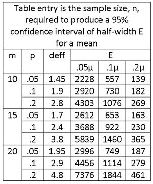
THE TABLE ENTRIES ARE NUMBER OF SAMPLE INTERVIEWS. TO OBTAIN THE NUMBER OF SAMPLE VILLAGES, DIVIDE BY THE NUMBER OF HOUSEHOLDS INTERVIEWED PER VILLAGE, m.

SUPPOSE THAT THE BUDGET CAN SUPPORT A SAMPLE OF h = 50 VILLAGES WITH m = 10 HOUSEHOLD INTERVIEWS IN EACH. THIS CORRESPONDS TO A TOTAL OF n = hm = 50 10 = 500 HOUSEHOLD INTERVIEWS. THE TABLE SHOWS THAT WITH THIS NUMBER OF HOUSEHOLD INTERVIEWS IT IS POSSIBLE TO ACHIEVE 95% CONFIDENCE INTERVALS OF HALF-WIDTH .2μ, BUT NOT .1μ.

CASE 4: STRATIFIED RANDOM SAMPLING, ESTIMATION OF THE POPULATION MEAN, μ, USING THE STRATUM-SIZE-WEIGHTED SAMPLE MEAN, AS THE ESTIMATOR FOR μ.

(A STRATIFIED RANDOM SAMPLE IS ONE IN WHICH THE POPULATION IS DIVIDED INTO NONOVERLAPPING GROUPS, CALLED STRATA, AND A SIMPLE RANDOM SAMPLE IS SELECTED FROM EACH STRATUM. STRATIFIED RANDOM SAMPLING IS USED FOR A NUMBER OF REASONS, AND CAN YIELD HIGHER PRECISION THAN SIMPLE RANDOM SAMPLING IF THE STRATA ARE INTERNALLY HOMOGENEOUS AND THE ALLOCATION OF THE SAMPLE TO THE STRATA IS APPROPRIATELY DONE. STRATIFICATION MAY BE APPLIED TO ELEMENTS OR TO CLUSTERS.)

ASSUMPTION: THE SAMPLE IS ALLOCATED TO THE STRATA IN PROPORTION TO THE STRATUM SIZE. IN THIS CASE THE PROBABILITY OF SELECTION FOR SECOND-STAGE UNITS IS A CONSTANT AND THE SAMPLE IS “SELF-WEIGHTING,” SO THAT THE ORDINARY SAMPLE MEAN IS UNBIASED.

LET

H = number of strata

H_i = number of elements in the i-th stratum (i.e., the stratum “size”)

N = total number of elements in all strata (i.e., the population size)

h_i = number of elements selected from the i-th stratum

n = total sample size (over all strata)

y_ij = response of the j-th unit in the i-th stratum

= mean for i-th stratum

(THE NOTATION IS SIMILAR TO THE CASE OF CLUSTER SAMPLING, BECAUSE THE STRUCTURE IS SIMILAR. IN CLUSTER SAMPLING, A SAMPLE OF CLUSTERS IS TAKEN AND ALL OF THE ELEMENTS WITHIN EACH SAMPLE CLUSTER ARE MEASURED. IN STRATIFIED SAMPLING, A SAMPLE IS SELECTED FROM EVERY STRATUM.)

THEN THE STRATUM-SIZE-WEIGHTED SAMPLE MEAN IS GIVEN BY

STRATIFIED SAMPLING USUALLY RESULTS IN A SMALLER VARIANCE FOR THE ESTIMATED MEAN THAN SIMPLE RANDOM SAMPLING. IF THE ALLOCATION OF THE SAMPLE TO THE STRATA IS PROPORTIONAL AND THE VARIANCES WITHIN STRATA ARE THE SAME, σ²_w, THEN

σ²_w/n

OR (1 - n/N) σ²_w/n IF THE fpc IS APPLICABLE.

IN THIS CASE, THE SAME FORMULA AS USED FOR DETERMINING SAMPLE SIZE IN SIMPLE RANDOM SAMPLING (CASE 1) MAY BE USED, REPLACING σ² IN THE FORMULAS BY σ²_w.

IN MOST APPLICATIONS, STRATA ARE SOMEWHAT INTERNALLY HOMOGENEOUS WITH RESPECT TO VARIABLES OF INTEREST, SO THE VALUE OF σ_w² IS LESS THAN σ² AND THERE IS AN INCREASE IN PRECISION OVER SIMPLE RANDOM SAMPLING.

THE VALUE OF THE DESIGN EFFECT, deff, IN THIS CASE IS deff = σ_w²/σ².

THE FORMULA FOR THE SAMPLE SIZE, IF THE fpc IS NOT RELEVANT, IS HENCE

WHERE deff = σ_w²/σ².

IF THE fpc IS RELEVANT, THE FORMULA IS

NOTE THAT THESE FORMULAS ASSUME THAT THE SAMPLE SIZE IN EACH STRATUM IS PROPORTIONAL TO THE STRATUM SIZE, AND THAT THE WITHIN-STRATUM VARIANCE IS THE SAME IN ALL STRATA. IF THESE ASSUMPTIONS DO NOT APPLY, THEN THE FORMULAS CHANGE (AND ARE MORE COMPLICATED).

FOR PROPORTIONAL ALLOCATION, THE SITUATION IS SIMILAR TO SIMPLE RANDOM SAMPLING, AND NO EXAMPLE WILL BE PRESENTED.

ESTIMATION FOR SUBPOPULATIONS

THE PRECEDING CONSIDERED THE CASE OF ESTIMATION OF CHARACTERISTICS OF THE POPULATION. IF ESTIMATES ARE DESIRED FOR SUBPOPULATIONS (E.G., BY GENDER, RACE, REGION, TREATMENT CATEGORY), THE SAME CALCULATIONS APPLY AS DESCRIBED ABOVE, BUT FOR EACH SUBPOPULATION OF INTEREST.

NOTE THAT IN MANY APPLICATIONS THE SAMPLE SIZE, n, REQUIRED TO ACHIEVE A DESIRED LEVEL OF PRECISION FOR A SUBPOPULATION IS THE SAME AS FOR THE TOTAL POPULATION. HENCE, IF THERE ARE A NUMBER OF SUBPOPULATIONS OF INTEREST, SAY n_sub, THE TOTAL SAMPLE SIZE REQUIRED WILL BE ABOUT EQUAL TO THE NUMBER OF SUBPOPULATIONS TIMES THAT SAMPLE SIZE, I.E., n n_sub.

FOR ESTIMATION OF CHARACTERISTICS OF SUBPOPULATIONS, THE SAMPLE IS STRATIFIED BY THE CHARACTERISTIC (OR CHARACTERISTICS) OF INTEREST. ORDINARY STRATIFICATION (CROSS-STRATIFICATION) IS PRACTICAL ONLY FOR A SMALL NUMBER OF VARIABLES OF STRATIFICATION. FOR A LARGE NUMBER OF VARIABLES OF STRATIFICATION, A PRACTICAL METHOD IS TO SET THE PROBABILITIES OF SELECTION SO THAT THE EXPECTED STRATUM SAMPLE SIZES ARE AS DESIRED FOR EACH VARIABLE OF STRATIFICATION SEPARATELY, I.E., TO USE MARGINAL STRATIFICATION.

SUMMARY

WE HAVE NOW CONSIDERED ESTIMATION OF THE SAMPLE MEAN FOR A SINGLE SAMPLE (OR GROUP), USING DIFFERENT SAMPLE DESIGNS. THE BASIC FORMULA IS THE SAME IN ALL CASES CONSIDERED.

IF THE SAMPLE SIZE, n, IS SMALL COMPARED TO THE POPULATION SIZE, N:

OTHERWISE

WHERE deff IS SPECIFIED IN THE FOLLOWING TABLE:

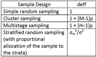
WE SHALL NOW CONSIDER ESTIMATION OF MORE COMPLEX QUANTITIES:

· SINGLE DIFFERENCE OF TWO GROUP MEANS

· DOUBLE DIFFERENCE OF FOUR GROUP MEANS

IN EVERY CASE, THE SAMPLE SIZE WILL BE ESTIMATED FROM AN EXPRESSION FOR THE SIZE OF A CONFIDENCE INTERVAL, WHICH DEPENDS ON THE VARIANCE OF AN ESTIMATOR OF THE QUANTITY OF INTEREST.

ESTIMATION OF (SINGLE) DIFFERENCES IN MEANS

ESTIMATES OF DIFFERENCES IN MEANS (OR PROPORTIONS) OF TWO GROUPS (DENOTED GROUP 1 AND GROUP 2) ARISE IN TWO MAIN WAYS:

· ESTIMATION OF DIFFERENCES IN MEANS BETWEEN SUBPOPULATIONS IN A GIVEN SURVEY ROUND (I.E., FOR A “CROSS-SECTIONAL” SURVEY CONDUCTED AT A POINT IN TIME), SUCH AS A COMPARISON BETWEEN TREATMENT AND CONTROL UNITS.

· ESTIMATION OF THE DIFFERENCE IN MEANS FOR THE SAME POPULATION (OR SUBPOPULATION) IN TWO DIFFERENT SURVEY ROUNDS (I.E., FOR A “LONGITUDINAL” SURVEY CONDUCTED AT TWO DIFFERENT POINT IN TIME).

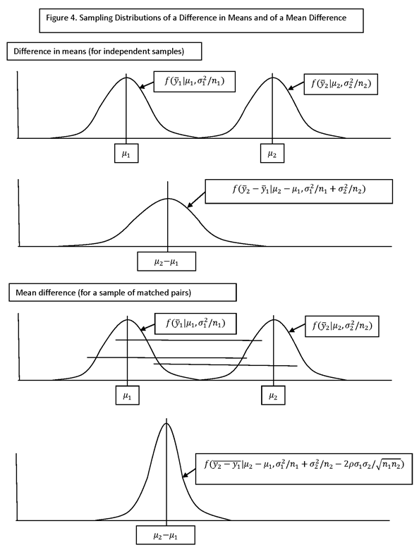
IF THE TWO GROUP MEANS ARE DENOTED BY AND , THEN THE VARIANCE OF THE DIFFERENCE, , IS, FOR SIMPLE RANDOM SAMPLING, GIVEN BY

WHERE ρ₁₂ DENOTES THE CORRELATION BETWEEN y₁ AND y₂.

FOR INDEPENDENT GROUPS, THE CORRELATION ρ₁₂ IS EQUAL TO ZERO.

IF THE SAMPLE SIZE IS THE SAME FOR THE TWO GROUPS, THE VARIANCE OF THE DIFFERENCE IS

IF, ALSO, THE VARIANCE IS THE SAME FOR THE TWO GROUPS (I.E., σ₁ = σ₂ = σ), THEN THIS BECOMES

(NOTE THAT IN COMPARING TREATMENT TO CONTROL, IF THE VARIANCE IS THE SAME IN THE TWO GROUPS, THEN USING THE SAME SAMPLE SIZE FOR EACH GROUP IS EFFICIENT. THE ASSUMPTION OF EQUAL VARIANCES AND EQUAL SAMPLE SIZES IS COMMON. OTHERWISE (IF NO INFORMATION IS AVAILABLE ABOUT THE VARIATION WITHIN THE TREATMENT AND CONTROL GROUPS), SINCE COMPARISON GROUPS TEND TO BE MORE HETEROGENEOUS THAN TREATMENT GROUPS, EFFICIENCY CONSIDERATIONS SUGGEST THAT THE SIZE OF THE COMPARISON GROUP SHOULD BE SOMEWHAT LARGER THAN THE TREATMENT GROUP.)

NOTE THAT THIS QUANTITY HAS THE SAME FORM AS THE VARIANCE OF A SINGLE SAMPLE MEAN, σ²/n, BUT MULTIPLIED BY A FACTOR, WHICH WE SHALL DENOTE AS varf. FOR THIS CASE (ESTIMATION OF A DIFFERENCE IN GROUP MEANS), THE VALUE OF varf IS 2(1 – ρ₁₂).

THE PRECEDING CASE IS FOR SIMPLE RANDOM SAMPLING. FOR OTHER SAMPLE DESIGNS (CLUSTER, MULTISTAGE, STRATIFIED), THE VARIANCE IS SIMPLY MULTIPLIED BY THE VALUE OF deff THAT IS APPROPRIATE FOR THAT DESIGN.

FOR DETERMINING SAMPLE SIZE FOR ESTIMATION OF DIFFERENCES, USE THE SAME FORMULAS PRESENTED EARLIER, SIMPLY REPLACING THE EXPRESSION FOR THE VARIANCE OF THE SAMPLE MEAN BY THE EXPRESSION FOR THE VARIANCE OF THE DIFFERENCE IN MEANS.

WE HENCE HAVE THE FOLLOWING RESULT.

IF THE SAMPLE SIZE, n, IS SMALL COMPARED TO THE POPULATION SIZE, N:

OTHERWISE

WHERE varf = 2(1 – ρ₁₂) AND deff IS SPECIFIED IN THE FOLLOWING TABLE:

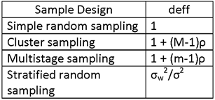
THE TERM “VARIANCE INFLATION FACTOR,” DENOTED BY VIF OR vif, IS SOMETIMES USED AS AN ALTERNATIVE TO deff varf. IF WE USE THE FACTOR vif TO DENOTE THE EXPRESSION deff varf, THEN THE EXPRESSION FOR THE SAMPLE SIZE IS GIVEN BY THE FOLLOWING, IN ALL CASES CONSIDERED SO FAR:

IF THE SAMPLE SIZE, n, IS SMALL COMPARED TO THE POPULATION SIZE, N:

OTHERWISE

WE SHALL NOW DISCUSS THE ROLE OF CORRELATION, ρ₁₂, BETWEEN THE TWO GROUPS FROM WHICH THE DIFFERENCE IS DERIVED.

CORRELATION MAY ARISE, FOR EXAMPLE, IN THE FOLLOWING WAYS:

IN THE SAME SURVEY ROUND, SAMPLE UNITS IN THE TWO GROUPS MAY BE MATCHED. FOR EXAMPLE, THE TWO GROUPS MIGHT BE TREATMENT AND CONTROL, WHERE EACH TREATMENT UNIT IS MATCHED TO A CONTROL UNIT (AT ANY LEVEL OF SAMPLING, E.G., AT THE VILLAGE LEVEL OR THE HOUSEHOLD LEVEL, IN A TWO-STAGE DESIGN).

IN SUCCESSIVE SURVEY ROUNDS, SAMPLING MAY BE CONDUCTED IN THE SAME SAMPLE UNIT (E.G., THE SAME VILLAGES, OR IN THE SAME HOUSEHOLDS).

NOTE THAT n IS THE SAMPLE SIZE FOR EACH OF THE TWO GROUPS FROM WHICH THE DIFFERENCE IS DERIVED. IF ρ₁₂ = 0, THEN THE VARIANCE OF THE DIFFERENCE IS 2σ²/n. TO ACHIEVE THE SAME LEVEL OF PRECISION AS FOR ESTIMATING A MEAN, THE SAMPLE SIZE WOULD HAVE TO BE TWICE AS LARGE, FOR EACH GROUP, OR FOUR TIMES AS LARGE IN ALL.

NOTE THAT SOME AUTHORS USE n TO DENOTE THE SAMPLE SIZE FOR ALL DESIGN GROUPS COMBINED. IN THAT CASE, THE FORMULAS GIVEN HERE ARE MULTIPLIED BY THE NUMBER OF DESIGN GROUPS (IN THIS CASE, TWO), IF THE GROUP SAMPLE SIZES ARE EQUAL.

IN THE ABSENCE OF CORRELATION BETWEEN THE GROUPS, THE SAMPLE-SIZE REQUIREMENTS FOR ESTIMATING DIFFERENCES IN MEANS ARE SUBSTANTIALLY GREATER THAN FOR ESTIMATING MEANS. THE REQUIRED SAMPLE SIZE CAN BE REDUCED SUBSTANTIALLY IF IT IS POSSIBLE TO INTRODUCE CORRELATION BETWEEN THE TWO GROUPS.

NOTE: FOR AN EXPERIMENTAL DESIGN INVOLVING RANDOMIZED ASSIGNMENT TO TREATMENT, MATCHING IS DONE PRIOR TO RANDOMIZED ASSIGNMENT TO TREATMENT. FOR A QUASI-EXPERIMENTAL DESIGN, MATCHING OF CONTROLS TO TREATMENT IS DONE AFTER SELECTION FOR TREATMENT.

NOTE ON CONCEPTUAL FRAMEWORK FOR TESTING HYPOTHESES ABOUT DIFFERENCES. IN ANY FINITE POPULATION, ANY TWO GROUPS ARE VIRTUALLY CERTAIN TO HAVE DIFFERENT MEANS, SO CONDUCTING A TEST OF THE HYPOTHESIS OF EQUALITY OF GROUP MEANS IN A FINITE POPULATION DOES NOT MAKE MUCH SENSE. IF A TEST OF THE HYPOTHESIS OF EQUALITY OF MEANS IS DONE, IT WOULD LIKELY BE SET IN A CONCEPTUAL FRAMEWORK IN WHICH THE TWO FINITE POPULATIONS REPRESENT SAMPLES FROM CONCEPTUALLY INFINITE POPULATIONS. (TESTING THE HYPOTHESIS THAT ONE GROUP MEAN IS LARGER OR SMALLER THAN ANOTHER DOES NOT PRESENT THIS PROBLEM.)

NOTE ON ASSUMPTION OF EQUALITY OF VARIANCES. IN MANY EXAMPLES INVOLVING TWO GROUP MEANS WE HAVE ASSUMED THAT σ₁² = σ₂². IN MANY APPLICATIONS THIS ASSUMPTION DOES NOT HOLD. FOR EXAMPLE, IN SAMPLING FOR PROPORTIONS THE TRUE VALUES OF THE PROPORTIONS WILL LIKELY DIFFER, AND SO THE VARIANCES WILL DIFFER ALSO. ALSO, IN APPLICATIONS INVOLVING INCOMES, THE VARIABILITY OF INCOME IS OFTEN PROPORTIONAL TO THE MEAN LEVEL. IN SUCH CASES, THE MORE GENERAL FORMULAS FOR THE SAMPLE SIZE SHOULD BE USED, NOT THE SIMPLIFIED ONES SHOWN HERE UNDER THE ASSUMPTION OF EQUALITY OF VARIANCES. (IN ALL CASES, THE MORE GENERAL FORMULAS FOR THE VARIANCE OF THE ESTIMATOR ARE SHOWN HERE.)

EXAMPLE

PROBLEM STATEMENT:

SINGLE-ROUND SURVEY, COMPARE TREATMENT TO CONTROL.

IF HAVE RANDOMIZED ASSIGNMENT TO TREATMENT, DON’T NEED SURVEYS AT TWO POINTS IN TIME (I.E., DON’T NEED A “BASELINE” SURVEY), SINCE RANDOMIZED ASSIGNMENT ASSURES THAT THE DISTRIBUTION OF ALL EXPLANATORY VARIABLES EXCEPT TREATMENT IS THE SAME FOR THE TREATMENT AND CONTROL SAMPLES.

MAY CONSIDER DESIGNS WITH AND WITHOUT MATCHING. FOR AN EXPERIMENTAL DESIGN, MATCHING IS DONE PRIOR TO RANDOMIZED ASSIGNMENT TO TREATMENT (A “MATCHED PAIRS” DESIGN). FOR A QUASI-EXPERIMENTAL DESIGN, MATCHING IS DONE AFTER ASSIGNMENT TO TREATMENT.

MATCHING IS GENERALLY DONE AT THE LOWEST LEVEL OF SAMPLING FOR WHICH USEFUL MATCHING DATA ARE AVAILABLE PRIOR TO THE SURVEY.

FIND REQUIRED SAMPLE SIZE FOR THE FOLLOWING:

E = .05σ, .1σ, .2σ (OR E = .05μ, .1μ, AND .2μ IF COEFFICIENT OF VARIATION (CV) = σ/μ = 1).

MATCHING VS. NON-MATCHING OF PRIMARY SAMPLE UNITS (VILLAGES). ASSUME MATCHING OF FIRST-STAGE UNITS (VILLAGES), FOR A TWO-STAGE SAMPLE DESIGN (SECOND-STAGE UNITS = HOUSEHOLDS). CORRELATION INTRODUCES BY MATCHING = ρ = .3.

INTRA-UNIT CORRELATION COEFFICIENT = icc = .05, .1, .2 (Note the change in notation; previously, ρ was used to denote the icc, and now it is used to denote the correlation associated with matching.)

HOUSEHOLD SAMPLE SIZE = m = 12.

SOLUTION:

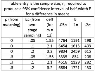
THE TABLE ENTRIES ARE NUMBERS OF HOUSEHOLDS. TO OBTAIN THE NUMBER OF SAMPLE VILLAGES, DIVIDE THE TABLE ENTRY BY THE NUMBER OF HOUSEHOLDS INTERVIEWED PER VILLAGE, m = 12.

OBSERVE THE SUBSTANTIAL DECREASE IN SAMPLE SIZE ASSOCIATED WITH MATCHING.

IF NONRESPONSE IS ANTICIPATED AT A RATE OF .1 FOR HOUSEHOLDS AND 0 FOR VILLAGES, INCREASE THE SAMPLE SIZE BY THE FACTOR 1/.9 = 1.11.

EXAMPLE

PROBLEM STATEMENT:

TWO-ROUND SURVEY, COMPARE BEFORE AND AFTER.

CONSIDER TWO CASES: (1) INDEPENDENT SURVEYS AT TWO POINTS IN TIME; AND (2) PANEL SURVEY IN WHICH ALL SAMPLE HOUSEHOLDS ARE INTERVIEWED IN BOTH SURVEYS.

MATCHING IS GENERALLY DONE AT THE LOWEST LEVEL OF SAMPLING FOR WHICH USEFUL MATCHING DATA ARE AVAILABLE PRIOR TO THE SURVEY.

FIND REQUIRED SAMPLE SIZE FOR THE FOLLOWING:

95% CONFIDENCE INTERVAL OF HALF-WIDTH E = .05σ, .1σ, .2σ (OR E = .05μ, .1μ, AND .2μ IF COEFFICIENT OF VARIATION (CV) = σ/μ = 1).

MATCHING VS. NON-MATCHING OF SUBUNITS (HOUSEHOLDS) OVER TIME. ASSUME THAT REINTERVIEW OF THE SAME HOUSEHOLDS IN BOTH SURVEYS INTRODUCES A CORRELATION OF ρ = .5.

INTRA-UNIT CORRELATION COEFFICIENT = icc = .05, .1, .2.

HOUSEHOLD SAMPLE SIZE = m = 12.

SOLUTION:

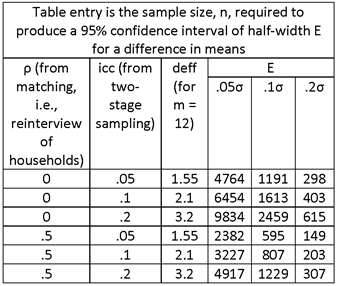
THE TABLE ENTRIES ARE NUMBERS OF HOUSEHOLDS; TO OBTAIN THE NUMBER OF SAMPLE VILLAGE, DIVIDE BY 12.

NOTE THAT THE TOP HALF OF THE TABLE IS EXACTLY THE SAME AS IN THE PREVIOUS EXAMPLE. IN BOTH CASES, THE DIFFERENCE IN MEANS IS BEING ESTIMATED FROM INDEPENDENT SAMPLES. IN THE PREVIOUS CASE, THE TWO SAMPLES WERE DIFFERENT GROUPS (TREATMENT AND CONTROL) AT THE SAME SURVEY ROUND (TIME). IN THIS CASE, THE TWO SAMPLES ARE THE SAME GROUP AT DIFFERENT ROUNDS (TIMES). IN THIS CASE, THE MATCHING ALLOWS FOR SMALLER SAMPLE SIZES THAN IN THE PREVIOUS CASE, SINCE THE CORRELATION ASSOCIATED WITH MATCHING IS GREATER (VIZ., .5 VS. .3).

OBSERVE THE SUBSTANTIAL DECREASE IN SAMPLE SIZE ASSOCIATED WITH MATCHING.

ASSUME NONRESPONSE FOR HOUSEHOLDS, BUT NOT FOR VILLAGES.

ASSUME .1 NONRESPONSE IN BASELINE (ROUND 1) SURVEY AND .1 ATTRITION IN SECOND ROUND SURVEY. TWO-ROUND RESPONSE RATE = .9 .9 = .81, OVERALL NONRESPONSE RATE = .19. TO ACCOUNT FOR THIS LEVEL OF NONRESPONSE, INCREASE THE SAMPLE SIZE BY FACTOR 1/.81 = 1.23.

ALTERNATIVE FORMULAS

THE FORMULA GIVEN ABOVE FOR SAMPLE SIZE IN THE CASE OF ESTIMATION OF SINGLE DIFFERENCES WAS

WHERE THE FORMULA FOR vif = deff varf WAS GIVEN IN THE CASE OF EQUAL VARIANCES AND SAMPLE SIZES FOR THE TWO DESIGN GROUPS (TREATMENT AND CONTROL, OR BEFORE AND AFTER).

IN THE CASE IN WHICH THE VARIANCES ARE NOT EQUAL AND/OR THE SAMPLE SIZES ARE NOT EQUAL, WE RETURN TO THE MORE GENERAL FORMULA FOR THE VARIANCE OF THE ESTIMATED DIFFERENCE IN MEANS:

IT IS CONVENIENT HERE TO CHANGE THE NOTATION A LITTLE. LET n DENOTE THE SAMPLE SIZE OF DESIGN GROUP 1 (I.E., n = n₁). LET US DEFINE r₂ (“r” FOR “ratio”) AS THE RATIO OF THE SAMPLE SIZES FOR DESIGN GROUP 2 RELATIVE TO THE SAMPLE SIZE FOR DESIGN GROUP 1, r₂ = n₂/n₁ = n₂/n.

THEN WE MAY WRITE THE PRECEDING EXPRESSION AS:

HENCE THE EXPRESSION FOR varf IS

AND THE EXPRESSION FOR vif IS

SOME AUTHORS DEFINE n AS THE SUM OF THE SAMPLE SIZES FOR BOTH DESIGN GROUPS (I.E., n = n₁ + n₂), AND DEFINE p AS THE PROPORTION OF THE SAMPLE ASSIGNED TO DESIGN GROUP 1, SO THAT n₁ = pn AND n₂ = (1-p)n. IN THIS CASE THE EXPRESSION FOR THE (TOTAL) SAMPLE SIZE IS

AND THE EXPRESSION FOR vif = deff varf IS

ESTIMATION OF DOUBLE DIFFERENCES

A COMMON DESIGN OCCURRING IN EVALUATION RESEARCH IS THE PRETEST-POSTTEST-COMPARISON-GROUP DESIGN, IN WHICH OBSERVATIONS ARE MADE ON TREATMENT AND COMPARISON (CONTROL) GROUPS AT TWO DIFFERENT POINTS IN TIME. (THE DESIGN MAY BE EITHER AN EXPERIMENTAL DESIGN OR A QUASI-EXPERIMENTAL DESIGN.)

THE STANDARD MEASURE OF IMPACT IS THE DOUBLE-DIFFERENCE MEASURE (SOMETIMES CALLED “DIFFERENCE IN DIFFERENCE” MEASURE), WHICH IS THE DIFFERENCE, BETWEEN THE TREATMENT AND COMPARISON GROUPS, OF THE DIFFERENCE IN MEANS AT THE TWO SURVEY TIMES.

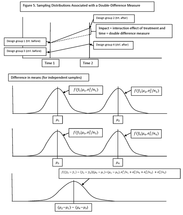
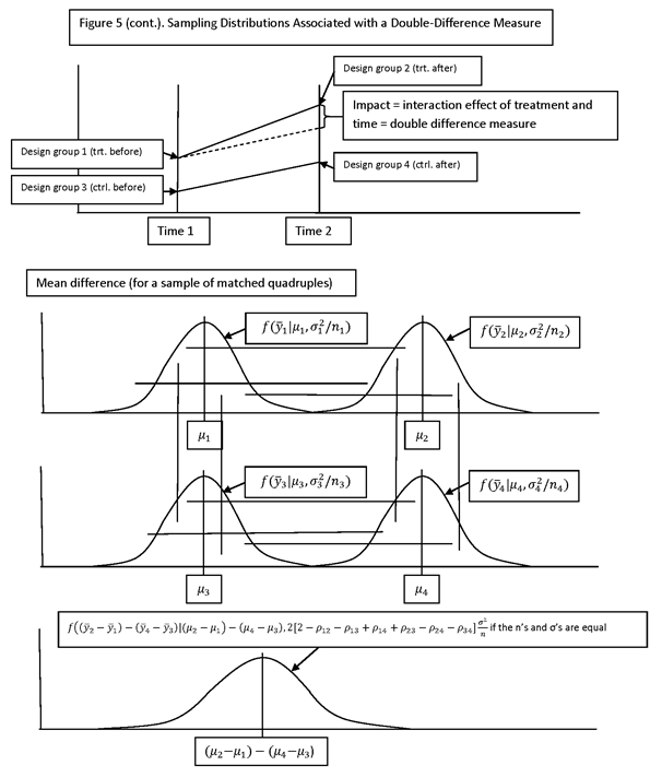
SUPPOSE THAT THE FOUR DESIGN GROUPS ARE DENOTED BY THE FOLLOWING INDICES:

GROUP 1: TREATMENT BEFORE

GROUP 2: TREATMENT AFTER

GROUP 3: CONTROL BEFORE.

GROUP 4: CONTROL AFTER

DENOTE THE POPULATION MEANS OF THE FOUR GROUPS BY μ₁, μ₂, μ₃ AND μ₄, AND THE SAMPLE MEANS BY , , AND .

THE DOUBLE-DIFFERENCE MEASURE (A POPULATION CHARACTERISTIC) IS

(μ₂ – μ₁) – (μ₄ – μ₃).

THE DOUBLE-DIFFERENCE ESTIMATOR (A SAMPLE STATISTIC) IS

FOR AN EXPERIMENTAL DESIGN IN WHICH TREATMENT IS ASSIGNED AT RANDOM, THE DOUBLE-DIFFERENCE ESTIMATOR IS AN UNBIASED ESTIMATE OF THE DOUBLE-DIFFERENCE MEASURE. OTHERWISE, ESTIMATION OF THE DOUBLE-DIFFERENCE MEASURE IS MORE COMPLICATED (E.G., USING REGRESSION ESTIMATORS OR MATCHING ESTIMATORS).

THE VARIANCE OF THE DOUBLE-DIFFERENCE ESTIMATOR IS GIVEN BY

WHERE σ_i² DENOTES THE VARIANCE OF ELEMENTS IN THE i-th DESIGN GROUP (I.E., OF y_i) AND ρ_ij DENOTES THE CORRELATION BETWEEN ELEMENTS OF THE i-th AND j-th GROUPS (I.E., BETWEEN y_i AND y_j).

IF ALL FOUR GROUPS ARE INDEPENDENT, ALL OF THE CORRELATIONS ARE ZERO.

IF THE VARIANCES AND SAMPLE SIZES ARE THE SAME FOR ALL FOUR GROUPS, THE PRECEDING FORMULA BECOMES

NOTE THAT THIS QUANTITY HAS THE SAME FORM AS THE VARIANCE OF A SINGLE SAMPLE MEAN, σ²/n, BUT MULTIPLIED BY A FACTOR, WHICH WE SHALL, AS BEFORE, CALL varf. FOR THIS CASE (ESTIMATION OF A DOUBLE DIFFERENCE IN GROUP MEANS), THE VALUE OF varf IS 2(2 – ρ₁₂ – ρ₁₃ + ρ₁₄ + ρ₂₃ – ρ₂₄ – ρ₃₄ ).

HENCE, FOR DETERMINING SAMPLE SIZE FOR ESTIMATION OF DOUBLE DIFFERENCES, USE THE SAME FORMULAS PRESENTED EARLIER, REPLACING (FOR EACH CASE) THE EXPRESSION FOR THE VARIANCE OF THE SAMPLE MEAN BY THE EXPRESSION FOR THE VARIANCE OF THE DOUBLE DIFFERENCE IN MEANS.

WE HENCE HAVE THE FOLLOWING RESULT.

IF THE SAMPLE SIZE, n, IS SMALL COMPARED TO THE POPULATION SIZE, N:

OTHERWISE

WHERE vif = deff varf, varf = varf IS 2(2 – ρ₁₂ – ρ₁₃ + ρ₁₄ + ρ₂₃ – ρ₂₄ – ρ₃₄ ) AND deff IS SPECIFIED IN THE FOLLOWING TABLE:

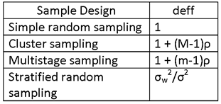
FOR DETERMINING SAMPLE SIZE FOR ESTIMATION OF DOUBLE DIFFERENCES, USE THE SAME FORMULAS PRESENTED EARLIER, SIMPLY REPLACING THE EXPRESSION FOR THE VARIANCE OF THE SAMPLE MEAN BY THE EXPRESSION FOR THE VARIANCE OF THE DOUBLE DIFFERENCE IN MEANS.

NOTE THAT n IS THE SAMPLE SIZE FOR EACH OF THE FOUR GROUPS FROM WHICH THE DIFFERENCE IS DERIVED. IF ALL OF THE ρ_ij = 0, THEN THE VARIANCE OF THE DIFFERENCE IS 4σ²/n. TO ACHIEVE THE SAME LEVEL OF PRECISION AS FOR ESTIMATING A MEAN, THE SAMPLE SIZE WOULD HAVE TO BE FOUR TIMES AS LARGE, FOR EACH GROUP, OR SIXTEEN TIMES AS LARGE IN ALL.

IN THE ABSENCE OF CORRELATION AMONG THE GROUPS, THE SAMPLE-SIZE REQUIREMENTS FOR ESTIMATING DOUBLE DIFFERENCES ARE SUBSTANTIALLY GREATER THAN FOR ESTIMATING MEANS. THE REQUIRED SAMPLE SIZE CAN BE REDUCED SUBSTANTIALLY IF IT IS POSSIBLE TO INTRODUCE CORRELATION AMONG THE FOUR GROUPS.

SOME COMMENTS ON THE CORRELATIONS

CORRELATIONS ARE INTRODUCED AMONG THE DESIGN GROUPS BY MATCHING. MATCHING MAY BE DONE AT VARIOUS SAMPLING LEVELS, E.G., AT THE HOUSEHOLD LEVEL OR THE VILLAGE LEVEL. IT IS DONE AT THE LOWEST PRACTICAL LEVEL OF SAMPLING. IN INTERNATIONAL DEVELOPMENT APPLICATIONS, MATCHING IS DONE AT THE ADMINISTRATIVE LEVEL (E.G., VILLAGE OR DISTRICT) FOR WHICH DATA ON USEFUL MATCH VARIABLES ARE AVAILABLE PRIOR TO THE SURVEY. A TYPICAL EXAMPLE IS MATCHING HOUSEHOLDS OVER TIME (I.E., INTERVIEWING THE SAME HOUSEHOLD IN SUCCESSIVE SURVEY ROUNDS) AND MATCHING VILLAGES OR DISTRICTS CROSS-SECTIONALLY AND OVER TIME (I.E., MATCHING THE VILLAGES IN THE BASELINE SURVEY AND USING THOSE SAME VILLAGES IN SUCCESSIVE SURVEY ROUNDS).

IN ORDER TO FORM A MATCHED QUADRUPLE (4-TUPLE) OF OBSERVATIONAL UNITS (E.G., HOUSEHOLDS), MATCHING WOULD HAVE TO BE DONE AT THAT LEVEL. IN INTERNATIONAL DEVELOPMENT APPLICATIONS, MATCHING OF QUADRUPLES IS UNUSUAL, SINCE HOUSEHOLD-LEVEL FRAMES ARE UNUSUAL AND BECAUSE MULTISTAGE SAMPLING IS USUALLY EMPLOYED.

FOR A PANEL SURVEY IN WHICH THE SAME HOUSEHOLDS ARE INTERVIEWED IN BOTH SURVEY ROUNDS, A “TYPICAL” VALUE FOR ρ₁₂ AND ρ₃₄ MIGHT BE .5.

FOR A TWO-STAGE SAMPLE IN WHICH VILLAGES ARE THE FIRST-STAGE SAMPLE UNITS AND HOUSEHOLDS ARE THE SECOND-STAGE SAMPLE UNITS, AND VILLAGES ARE MATCHED ON A VARIETY OF VARIABLES RELATED TO OUTCOMES OF INTEREST (E.G., RELEVANT SOCIOECONOMIC OR AGRICULTURAL VARIABLES), A TYPICAL VALUE FOR ρ₁₃ AND ρ₂₄ MIGHT BE .3.

THE VALUES OF ρ₂₃ AND ρ₁₄ MUST BE SPECIFIED SO THAT THE CORRELATION MATRIX OF (y₁, y₂, y₃, y₄) IS NONSINGULAR (POSITIVE DEFINITE). REASONABLE VALUES ARE ρ₂₃ = ρ₂₄ ρ₃₄ AND ρ₁₄ = ρ₁₂ ρ₁₃. (SEE THE SAMPLE-SIZE PROGRAM JGCSampleSizeProgramV53_20130917.accde FOR THE RATIONALE FOR THESE VALUES.)

IF THE SAME HOUSEHOLDS ARE INTERVIEWED IN SUCCESSIVE ROUNDS, AND/OR IF MATCHING IS DONE BETWEEN TREATMENT AND CONTROL UNITS, THE VARIANCE OF THE ESTIMATE MAY BE SUBSTANTIALLY REDUCED. THIS REDUCTION IS VERY IMPORTANT FOR IMPACT EVALUATIONS IN INTERNATIONAL DEVELOPMENT APPLICATIONS, WHERE THE SAMPLE SIZES ARE USUALLY NOT LARGE. USING THESE MATCHING METHODS CAN SUBSTANTIALLY REDUCE THE SAMPLE SIZE REQUIRED TO ACHIEVE A SPECIFIED LEVEL OF PRECISION.

AS MENTIONED, THE DOUBLE-DIFFERENCE ESTIMATOR MAY BE BIASED FOR A QUASI-EXPERIMENTAL DESIGN, AND BETTER (REDUCED-BIAS) ESTIMATORS ARE USED (E.G., REGRESSION ESTIMATORS, MATCHING ESTIMATORS) TO ESTIMATE THE POPULATION DOUBLE-DIFFERENCE MEASURE. NEVERTHELESS, THE VARIANCE OF THE DOUBLE-DIFFERENCE ESTIMATOR IS USUALLY USED AS THE BASIS FOR ESTIMATING SAMPLE SIZE.

OTHER ESTIMATORS

IF THERE IS REASON TO BELIEVE THAT THE PRECISION OF THE ESTIMATOR MAY BE SUBSTANTIALLY BETTER THAN THE PRECISION OF THE DOUBLE DIFFERENCE ESTIMATOR, THEN AN APPROPRIATE ADJUSTMENT SHOULD BE MADE TO deff TO REFLECT THIS. DESCRIPTIVE SURVEYS SOMETIMES MAKE USE OF SIMPLE RATIO AND REGRESSION ESTIMATORS, BUT THESE ARE USUALLY DESIGN-BASED ESTIMATORS OF BASIC OUTCOME MEASURES, NOT OF SINGLE OR DOUBLE DIFFERENCES. MORE COMPLEX ESTIMATORS WILL BE CONSIDERED LATER, IN ADDRESSING ANALYTICAL SURVEYS.

IN GENERAL, THE FORMULAS FOR ESTIMATING SAMPLE SIZE USING OTHER ESTIMATORS ARE THE SAME AS DESCRIBED ABOVE, WHERE THE TERM deff varf σ² REFERS TO THE VARIANCE OF WHATEVER QUANTITY IS BEING ESTIMATED.

EXAMPLE

PROBLEM STATEMENT:

FOR A TWO-ROUND SURVEY, ESTIMATE THE SAMPLE SIZE REQUIRED UNDER THE FOLLOWING CONDITIONS.

95% CONFIDENCE INTERVALS OF HALF-WIDTH, E, OF .05, .1σ AND .2σ.

FIRST-STAGE SAMPLE OF VILLAGES AND SECOND-STAGE SAMPLE OF HOUSEHOLDS WITHIN VILLAGES.

HOUSEHOLD SAMPLE SIZE OF m = 12 PER SAMPLE VILLAGE.

VARIABLES HAVING INTRA-VILLAGE CORRELATION COEFFICIENTS OF icc = .05, .1 AND .2.

MATCHING OF HOUSEHOLDS: INTERVIEW THE SAME HOUSEHOLDS IN BOTH SURVEY ROUNDS, CORRELATIONS ρ₁₂ = ρ₃₄ = .5.

MATCHING OF VILLAGES, CORRELATIONS ρ₁₃ = ρ₂₄ = .3.

(ASSUMED VALUES FOR CORRELATIONS BETWEEN OTHER DESIGN GROUPS: ρ₁₄ = ρ₂₃ = .3 .5 = .15.)

SOLUTION:

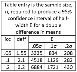
TABLE ENTRIES ARE NUMBERS OF SAMPLE HOUSEHOLDS; DIVIDE BY m = 12 TO OBTAIN NUMBERS OF SAMPLE VILLAGES.

ASSUME NONRESPONSE FOR HOUSEHOLDS, BUT NOT FOR VILLAGES.

SUMMARY

IN ALL CASES, THE FOLLOWING FORMULAS MAY BE USED TO ESTIMATE SAMPLE SIZE FOR DESCRIPTIVE SURVEYS.

IF THE SAMPLE SIZE, n, IS SMALL COMPARED TO THE POPULATION SIZE, N:

OTHERWISE

WHERE vif = deff varf, deff IS SPECIFIED IN THE FOLLOWING TABLE:

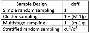
AND varf IS SPECIFIED IN THE FOLLOWING TABLE:

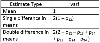
MORE COMPLEX ESTIMATORS MAY ARISE IN THE ANALYSIS, SUCH AS RATIO AND REGRESSION ESTIMATORS, BUT THEY ARE RARELY CONSIDERED FOR PRELIMINARY SAMPLE-SIZE ESTIMATION FOR DESCRIPTIVE SURVEYS. (REGRESSION ESTIMATORS WILL BE CONSIDERED IN SAMPLE-SIZE ESTIMATION FOR ANALYTICAL SURVEYS.)

IN SOME INSTANCES, WHERE LITTLE IS KNOWN ABOUT A POPULATION, A LISTING SURVEY IS CONDUCTED TO CONSTRUCT A SAMPLE FRAME, INCLUDING INFORMATION ON VARIANCES OF KEY VARIABLES AND INFORMATION ON VARIABLES THAT MAY BE USEFUL IN DESIGN.

4. SAMPLE SIZE ESTIMATION FOR ANALYTICAL SURVEYS

GOALS OF AN ANALYTICAL SURVEY:

· ESTIMATION OF THE EFFECT (“IMPACT”) OF A PROGRAM INTERVENTION ON A POPULATION

· ESTIMATION OF RELATIONSHIP OF IMPACT TO EXPLANATORY VARIABLES

DIFFERENCES FROM DESCRIPTIVE SURVEYS

· ESTIMATES ARE MODEL-BASED (OR MODEL-ASSISTED), NOT DESIGN-BASED

· MANY VARIABLES ARE ASSUMED TO BE RANDOM, NOT FIXED (“RANDOM EFFECTS,” “FIXED EFFECTS,” “MIXED MODEL”)

· CONSIDERABLE USE OF REGRESSION ESTIMATORS AND OTHER COMPLEX ESTIMATORS (SUCH AS MATCHING ESTIMATORS AND TWO-STEP ESTIMATORS)

NOTE THAT THE RATIO AND REGRESSION ESTIMATORS THAT OCCUR IN DESCRIPTIVE SURVEYS ARE SIMPLE MODELS USED TO INCREASE PRECISION, AND DIFFER SUBSTANTIALLY FROM THE REGRESSION MODELS USED IN THE ANALYSIS OF ANALYTICAL-SURVEY DATA.

SAMPLE SIZE DEPENDS ON:

· THE ESTIMATOR OF INTEREST (E.G., A MEAN, DIFFERENCE IN MEANS, OR DOUBLE-DIFFERENCE IN MEANS)

· THE TEST PARAMETERS (SIZE (“SIGNIFICANCE LEVEL”), POWER AND MINIMUM DETECTABLE EFFECT)

· POPULATION CHARACTERISTICS (STANDARD DEVIATIONS, INTERNAL HOMOGENEITY OF POTENTIAL SAMPLING UNITS (E.G., VILLAGES) OR STRATA, SUBPOPULATIONS OF INTEREST)

· SURVEY COSTS (E.G., RELATIVE COST OF SAMPLING A VILLAGE VS. SAMPLING A HOUSEHOLD)

· SURVEY DESIGN (E.G., WHETHER TO USE SIMPLE RANDOM SAMPLING, CLUSTER SAMPLING, MULTISTAGE SAMPLING OR STRATIFIED SAMPLING)

MUCH OF WHAT WAS DISCUSSED FOR ESTIMATING SAMPLE SIZE FOR DESCRIPTIVE SURVEYS PERTAINS TO ANALYTICAL SURVEYS, SUCH AS THE BASIC TYPES OF SURVEY DESIGN. AS BEFORE, IT IS ASSUMED THAT THE SAMPLE SIZES ARE SUFFICIENTLY LARGE THAT THE SAMPLE MEAN IS A GOOD ESTIMATE OF THE POPULATION MEAN, AND IS APPROXIMATELY NORMALLY DISTRIBUTED.

AS BEFORE, WE WILL CONSIDER THE FOLLOWING FOUR DESIGNS:

· SIMPLE RANDOM SAMPLING

· SINGLE-STAGE CLUSTER SAMPLING

· TWO-STAGE SAMPLING (CLUSTER SAMPLING WITH SUBSAMPLING)

· STRATIFIED SAMPLING

IN THE FOLLOWING SITUATIONS:

· SINGLE ROUND (TIME) OF SAMPLING, NO SUBPOPULATIONS OF INTEREST

· SINGLE ROUND OF SAMPLING, SUBPOPULATIONS (E.G., TREATED VS. UNTREATED, MALES VS FEMALES, REGIONS, TREATMENT MODALITIES)

· TWO ROUNDS OF SAMPLING

FOR ANALYTICAL SURVEYS, ATTENTION FOCUSES ON TESTS OF HYPOTHESES ABOUT PARAMETERS OF INTEREST. THE TESTS OF HYPOTHESES TO BE CONSIDERED ARE:

· TESTS OF HYPOTHESES ABOUT MEANS

· TESTS OF HYPOTHESES ABOUT PROPORTIONS

· TESTS OF HYPOTHESES ABOUT DIFFERENCES (SINGLE DIFFERENCES, DOUBLE DIFFERENCES)

TESTS OF HYPOTHESES ABOUT TOTALS RARELY ARISE IN ANALYTICAL SURVEYS, AND WILL NOT BE CONSIDERED HERE.

THE FOCUS OF THE PRESENTATION WILL BE ESTIMATION OF SAMPLE SIZE, GIVEN A SPECIFICATION OF A DESIRED MINIMUM DETECTABLE EFFECT. IN MANY INSTANCES, IT IS DESIRED TO DETERMINE THE MINIMUM DETECTABLE EFFECT, GIVEN THE SAMPLE SIZE. BOTH PROBLEMS ARE SOLVED USING THE SAME FORMULA.

BASIC APPROACH:

THE SAMPLE SIZE WILL BE DETERMINED TO PROVIDE A SPECIFIED LEVEL OF POWER FOR A TEST OF HYPOTHESIS ABOUT A QUANTITY OF INTEREST, SUCH AS:

· THE POPULATION MEAN (OR PROPORTION) EXCEEDS (OR EQUALS) A SPECIFIED VALUE

· THE DIFFERENCE IN MEANS BETWEEN TWO POPULATION GROUPS EXCEEDS A SPECIFIED VALUE

· A DOUBLE DIFFERENCE IN POPULATION MEANS EXCEEDS A SPECIFIED VALUE

THE SPECIFIED VALUE REFERRED TO IS CALLED THE “MINIMUM DETECTABLE EFFECT.” THE POWER OF THE TEST IS THE PROBABILITY OF DETECTING THE MINIMUM DETECTABLE EFFECT, I.E., OF ACCEPTING THE HYPOTHESIS THAT THE QUANTITY OF INTEREST EXCEEDS THE MINIMUM DETECTABLE EFFECT, WHEN IT IN FACT DOES.

SOME TERMINOLOGY AND NOTATION:

TEST OF HYPOTHESIS: DECIDE BETWEEN TWO HYPOTHESES, A NULL HYPOTHESIS (H₀) AND AN ALTERNATIVE HYPOTHESIS (H₁).

TYPE I ERROR: DECIDING H₁ IS TRUE WHEN IN FACT H₀ IS TRUE

TYPE II ERROR: DECIDING H₀ IS TRUE WHEN IN FACT H₁ IS TRUE

(THE HYPOTHESES ARE USUALLY NAMED SO THAT THE TYPE I ERROR IS MORE SERIOUS.)

P(TYPE I ERROR) = α = SIZE OF THE TEST (SOMETIMES CALLED THE SIGNIFICANCE LEVEL OF THE TEST)

P(TYPE II ERROR) = β

IF THE ALTERNATIVE HYPOTHESIS IS PARAMETERIZED BY A PARAMETER, θ, THEN β IS A FUNCTION OF θ. A PLOT OF β(θ) IS CALLED THE OPERATING CHARACTERISTIC CURVE, OR “OC” CURVE. THE FUNCTION 1 – β(θ) = P(REJECT H₀ | θ) IS CALLED THE POWER FUNCTION.

CRITICAL REGION OF A TEST: THE CONDITIONS UNDER WHICH THE NULL HYPOTHESIS (H₀) IS REJECTED.

D = MINIMUM DETECTABLE EFFECT I.E., THE MINIMUM EFFECT (ASSUMED TO BE POSITIVE) THAT IT IS DESIRED TO DETECT WITH HIGH PROBABILITY. FOR EXAMPLE, IF H₀: mean = 0 and H₁: mean >=D, THEN THE MINIMUM DETECTABLE EFFECT IS D.

NOTE THAT THE PRECEDING CASES REPRESENT “ONE-SIDED” TESTS OF HYPOTHESES. THE REASON FOR THIS IS THAT IN EVALUATION RESEARCH THE SIGN OF AN EFFECT IS USUALLY SPECIFIED. FOR EXAMPLE, IT IS DESIRED AND EXPECTED THAT A JOB TRAINING PROGRAM WILL INCREASE EMPLOYMENT AND EARNINGS, AND IT IS OF INTEREST TO TEST WHETHER AN INCREASE OCCURRED.

THIS SITUATION DIFFERS FROM THE SITUATION IN TESTING THE SIGNIFICANCE OF REGRESSION COEFFICIENTS, WHERE THE SIGN OF A COEFFICIENT MAY OFTEN BE OF EITHER SIGN, DEPENDING ON WHAT OTHER VARIABLES ARE INCLUDED IN THE REGRESSION MODEL.

IF THE SIGN OF THE EFFECT OF INTEREST IS IN DOUBT, THEN A TWO-SIDED TEST SHOULD BE USED. THE TWO-SIDED CASE REQUIRES A LARGER SAMPLE SIZE (FOR THE SAME POWER) THAN THE ONE-SIDED CASE (SO A “CONSERVATIVE” APPROACH WOULD BE TO USE THE TWO-SIDED TEST).

IN EVALUATION RESEARCH, THE PARTICULAR FINITE POPULATION BEING SURVEYED IS NOT OF DIRECT INTEREST. WHAT IS OF INTEREST IS THE EFFECT OF A PROCESS (SUCH AS A TRAINING PROGRAM, OR A POLICY CHANGE) ON THE POPULATION. THE POPULATION AT HAND IS CONSIDERED TO BE A SINGLE SAMPLE FROM A CONCEPTUALLY INFINITE POPULATION, WHICH MAY BE AFFECTED BY THE PROGRAM INTERVENTION (TREATMENT). FOR THIS REASON, THE SIZE, N, OF THE POPULATION IS (USUALLY) NOT RELEVANT.

THE SIZE OF THE POPULATION OF FIRST-STAGE UNITS MAY BE OF INTEREST, IN CERTAIN SITUATIONS (FIXED-EFFECT MODELS, WHICH ARE NOT CONSIDERED HERE).

CASE 5: SIMPLE RANDOM SAMPLING, TEST OF HYPOTHESIS THAT THE POPULATION MEAN, μ, EXCEEDS A VALUE, D, USING THE SAMPLE MEAN, , AS THE ESTIMATOR FOR μ.

USING THE STANDARD (NEYMAN-PEARSON, LIKELIHOOD RATIO) APPROACH TO HYPOTHESIS TESTING, THE UNIFORMLY MOST POWERFUL TEST OF THE HYPOTHESIS THAT μ <= D VERSUS THE ALTERNATIVE HYPOTHESIS THAT μ>D IS BASED (IN SAMPLING FROM A WIDE CLASS OF DISTRIBUTIONS) ON THE SAMPLE MEAN, AND THE CRITICAL REGION IS DEFINED AS ALL VALUES FOR WHICH THE STANDARDIZED MEAN

EXCEEDS THE VALUE z_α, THE 1 – α PERCENTILE OF THE STANDARD NORMAL DISTRIBUTION (I.E., THE VALUE BELOW WHICH A STANDARD NORMAL RANDOM VARIABLE HAS PROBABILITY 1 – α OF OCCURRENCE).

(NOTE THAT z_α IS USED INSTEAD OF z_α/2 SINCE IT IS ASSUMED THAT A ONE-SIDED TEST IS BEING USED. FOR TWO-SIDED TESTS REPLACE z_α BY z_α/2 IN THE FOLLOWING DISCUSSION.)

THAT IS, REJECT H₀ IF

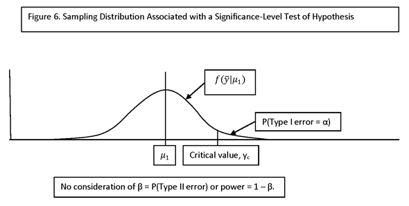
NOW, IF THE VALUE OF THE POPULATION MEAN, μ, IS D, THEN THE POWER OF THIS TEST IS

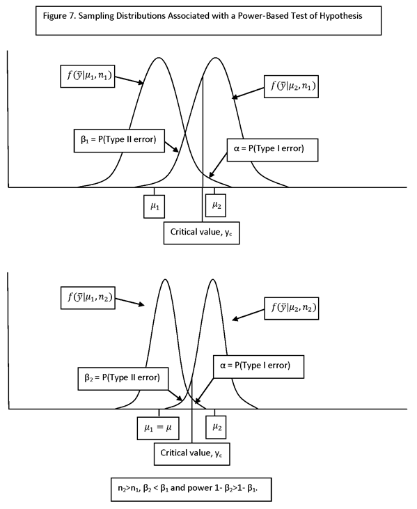
PROCEEDING AS BEFORE (IN THE CASE OF DESCRIPTIVE SURVEYS), WE HAVE

THE EXPRESSION FOR 1- β IS EQUIVALENT TO:

OR, SINCE

IS A STANDARDIZED NORMAL DEVIATE,

OR (SINCE ),

OR, SINCE

SOLVING FOR n WE OBTAIN

THIS IS THE FUNDAMENTAL FORMULA FOR ESTIMATING SAMPLE SIZE FOR ANALYTICAL SURVEYS, USING STATISTICAL POWER ANALYSIS. (NOTE THAT z_α IS REPLACED BY z_α/2 FOR TWO-SIDE TESTS.)

THE PRECEDING FORMULA APPLIES TO THE CASE OF SIMPLE RANDOM SAMPLING AND TESTING AN HYPOTHESIS ABOUT THE POPULATION MEAN.

FOR ALL OF THE SAME CASES CONSIDERED FOR DESCRIPTIVE SURVEYS, THE SAMPLE SIZE FOR ANALYTICAL SURVEYS IS OBTAINED SIMPLY BY MULTIPLYING THE VARIANCE σ² IN THE PRECEDING EXPRESSION BY THE FACTORS deff AND varf THAT ARE APPROPRIATE FOR THE SAMPLE DESIGN AND ESTIMATOR TYPE, AS SHOWN PREVIOUSLY FOR DESCRIPTIVE SURVEYS.

NOTE THAT THESE FORMULAS APPLY TO DESIGN-BASED ESTIMATES, NOT TO MODEL-BASED ESTIMATES, WHICH WILL BE CONSIDERED LATER.

FOR ANALYTICAL SURVEYS, THE INFINITE-POPULATION CONCEPTUAL FRAMEWORK APPLIES, SO THE fpc IS NOT RELEVANT.

HENCE, IN ALL CASES CONSIDERED, THE FORMULA FOR ESTIMATING SAMPLE SIZE FOR ANALYTICAL SURVEYS IS

WHERE vif = deff varf, AND THE VALUES FOR deff AND varf ARE AS SPECIFIED PREVIOUSLY, FOR DESCRIPTIVE SURVEYS.

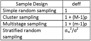
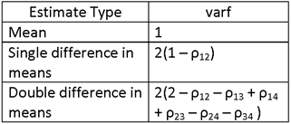
IT IS OF INTEREST TO COMPARE THE FORMULA FOR SAMPLE SIZE FOR ANALYTICAL SURVEYS (BASED ON STATISTICAL POWER ANALYSIS) TO THAT FOR DESCRIPTIVE SURVEYS (BASED ON PRECISION ANALYSIS). THE TWO FORMULAS PRODUCE THE SAME SAMPLE SIZE IF E=D AND IF THE QUANTITY INVOLVING z IS THE SAME. FOR DESCRIPTIVE SURVEYS THIS QUANTITY IS z_α. FOR ANALYTICAL SURVEYS THIS QUANTITY IS EITHER z_α + z_β or z_α/2 + z_β, DEPENDING ON WHETHER A ONE-SIDED TEST OR TWO-SIDED TEST OF HYPOTHESIS IS USED. FOR A ONE-SIDED TEST, THE SAMPLE SIZE WOULD ALWAYS BE HIGHER FOR THE ANALYTICAL SURVEY. FOR A TWO-SIDED TEST, THE SAMPLE SIZE WOULD BE THE SAME IF z_α = z_α/2 + z_β.

EXAMPLE

TEST OF HYPOTHESIS CONCERNING A MEAN.

PROBLEM STATEMENT:

FOR A SINGLE-ROUND SURVEY, ESTIMATE THE SAMPLE SIZE REQUIRED UNDER THE FOLLOWING CONDITIONS.

ESTIMATOR: SAMPLE MEAN.

MINIMUM DETECTABLE EFFECT, E, OF .05, .1σ AND .2σ.

TEST PARAMETERS: α = .05, β= .9 (I.E., POWER = 1 – β = .9)

FIRST-STAGE SAMPLE OF VILLAGES AND SECOND-STAGE SAMPLE OF HOUSEHOLDS WITHIN VILLAGES

HOUSEHOLD SAMPLE SIZE OF m = 12 PER SAMPLE VILLAGE.

VARIABLES HAVING INTRA-VILLAGE CORRELATION COEFFICIENTS OF icc = .05, .1 AND .2.

SOLUTION:

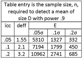
EXAMPLE

TEST OF HYPOTHESIS CONCERNING A DIFFERENCE IN MEANS.

PROBLEM STATEMENT:

FOR A SINGLE-ROUND SURVEY, ESTIMATE THE SAMPLE SIZE REQUIRED UNDER THE FOLLOWING CONDITIONS.

ESTIMATOR: SINGLE DIFFERENCE IN MEANS BETWEEN A TREATMENT GROUP AND A CONTROL GROUP.

MINIMUM DETECTABLE EFFECT, E, OF .05, .1σ AND .2σ.

TEST PARAMETERS: α = .05, β= .9 (I.E., POWER = 1 – β = .9)

FIRST-STAGE SAMPLE OF VILLAGES AND SECOND-STAGE SAMPLE OF HOUSEHOLDS WITHIN VILLAGES

HOUSEHOLD SAMPLE SIZE OF m = 12 PER SAMPLE VILLAGE.

VARIABLES HAVING INTRA-VILLAGE CORRELATION COEFFICIENTS OF icc = .05, .1 AND .2.

MATCHING OF VILLAGES, CORRELATION ρ = .3.

ESTIMATE THE SAMPLE SIZE WITH AND WITHOUT MATCHING.

SOLUTION:

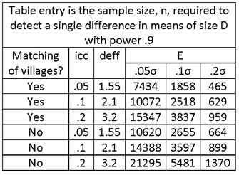
THERE ARE TWO MAJOR POINTS TO NOTE ABOUT THIS TABLE. FIRST, THE SAMPLE SIZES FOR NO MATCHING ARE DOUBLE THOSE FOR THE PREVIOUS EXAMPLE. THIS IS BECAUSE THE VARIANCE OF A DIFFERENCE IN MEANS (OF THE SAME SAMPLE SIZE AND ELEMENT VARIANCE) IS TWICE THE VARIANCE OF A SINGLE MEAN. THE SECOND IS THAT IF MATCHING OF VILLAGES IS DONE, THERE IS A SUBSTANTIAL REDUCTION IN THE REQUIRED SAMPLE SIZE.

EXAMPLE

TEST OF HYPOTHESIS CONCERNING A DOUBLE DIFFERENCE IN MEANS.

PROBLEM STATEMENT:

ESTIMATOR: DOUBLE DIFFERENCE IN MEANS (TREATMENT AND CONTROL, BEFORE AND AFTER).

FOR A TWO-ROUND SURVEY, ESTIMATE THE SAMPLE SIZE REQUIRED UNDER THE FOLLOWING CONDITIONS.

MINIMUM DETECTABLE EFFECT, E, OF .05, .1σ AND .2σ.

TEST PARAMETERS: α = .05, β= .9 (I.E., POWER = 1 – β = .9)

FIRST-STAGE SAMPLE OF VILLAGES AND SECOND-STAGE SAMPLE OF HOUSEHOLDS WITHIN VILLAGES

HOUSEHOLD SAMPLE SIZE OF m = 12 PER SAMPLE VILLAGE.

VARIABLES HAVING INTRA-VILLAGE CORRELATION COEFFICIENTS OF icc = .05, .1 AND .2.

IF MATCH HOUSEHOLDS: INTERVIEW THE SAME HOUSEHOLDS IN BOTH SURVEY ROUNDS, CORRELATIONS ρ₁₂ = ρ₃₄ = .5.

IF MATCH VILLAGES, CORRELATION ρ₁₃ = ρ₂₄ = .3.

(ASSUMED VALUES FOR CORRELATIONS BETWEEN OTHER DESIGN GROUPS: ρ₁₄ = ρ₂₃ = (.3) (.5) = .15.)

DETERMINE THE SAMPLE SIZE WITH AND WITHOUT MATCHING (OF HOUSEHOLDS AND/OR VILLAGES).

SOLUTION:

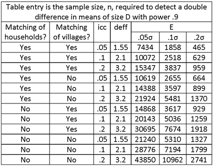
THERE ARE TWO MAJOR POINTS TO NOTE ABOUT THIS TABLE. FIRST, THE SAMPLE SIZES FOR NO MATCHING ARE DOUBLE THOSE FOR THE PREVIOUS EXAMPLE. THIS IS BECAUSE THE VARIANCE OF A DOUBLE DIFFERENCE IN MEANS (OF THE SAME SAMPLE SIZE AND ELEMENT VARIANCE) IS TWICE THE VARIANCE OF A SINGLE DIFFERENCE IN MEANS. THE SECOND IS THAT IF MATCHING OF VILLAGES AND HOUSEHOLDS IS DONE, THERE IS A SUBSTANTIAL REDUCTION IN THE REQUIRED SAMPLE SIZE. THIS IS A VERY IMPORTANT POINT. IN THE ABSENCE OF MATCHING, THE SAMPLE SIZES REQUIRED TO DETECT DIFFERENCES IS SUBSTANTIALLY LARGER THAN IF MATCHING IS DONE.

THE POWER FUNCTION

AS MENTIONED, BECAUSE OF THE UNCERTAINTY IN THE VALUES OF THE POPULATION PARAMETERS, AND THE FACT THAT THEY DIFFER FOR DIFFERENT VARIABLES OF INTEREST, IT IS USEFUL TO CALCULATE SAMPLE SIZES FOR A RANGE OF VALUES OF EACH ONE.

A STANDARD WAY OF SUMMARIZING POWER IS TO CONSTRUCT A TABLE OR GRAPH SHOWING THE POWER FUNCTION, WHICH IS THE POWER EXPRESSED AS A FUNCTION OF THE EFFECT (OR “MINIMAL DETECTABLE EFFECT”). THE POWER FUNCTION MAY BE DISPLAYED IN A TABLE OR A GRAPH, AS A POWER CURVE. IT IS USUALLY SHOWN AS A FUNCTION OF SAMPLE SIZE, AND PERHAPS ALSO OF THE SIZE (α) OF THE TEST.

THE PRECEDING TABLE IS AN EXAMPLE OF A POWER FUNCTION (CALCULATED FOR THREE EFFECT SIZES).

HERE IS AN EXAMPLE OF A TABLE SHOWING A POWER FUNCTION.

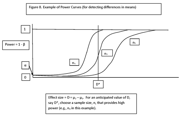
THE POWER FUNCTION IS THE PROBABILITY OF REJECTING THE NULL HYPOTHESIS FOR A SPECIFIED EFFECT SIZE. A PLOT OF THE PROBABILITY OF ACCEPTING THE NULL HYPOTHESIS AS A FUNCTION OF EFFECT SIZE IS CALLED THE OPERATING CHARACTERISTIC CURVE, OR OC CURVE. THE OC CURVE IS USED IN QUALITY CONTROL APPLICATIONS.

THE RECEIVER OPERATING CHARACTERISTIC (ROC) CURVE

IN DETERMINING SAMPLE SIZE, ONE APPROACH IS TO SPECIFY VALUES FOR α AND β AND DETERMINE THE CORRESPONDING SAMPLE SIZE. TO ACCOMMODATE BUDGETARY CONSTRAINTS, ANOTHER APPROACH IS TO SET A VALUE FOR α AND DETERMINE THE VALUE OF β CORRESPONDING TO A SPECIFIED SAMPLE SIZE. IF THE POWER, 1 – β, FOR DETECTING A SPECIFIED EFFECT IS ADEQUATE, THE SURVEY PROCEEDS.

IT IS IMPORTANT TO RECOGNIZE THAT THERE IS AN INVERSE RELATIONSHIP BETWEEN THE VALUES OF α AND β. FIGURE 9 ILLUSTRATES THE SITUATION.

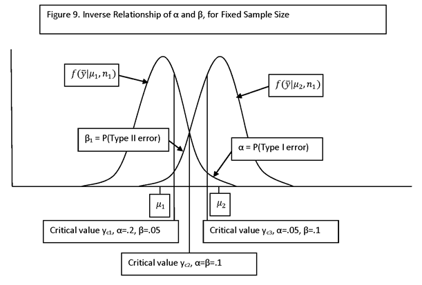
FIGURE 10 PRESENTS A RECEIVER OPERATING CHARACTERISTIC, OR ROC, CURVE. THE ROC CURVE IS A PLOT OF 1 – α (OR “TRUE POSITIVE RATE” OR “SENSITIVITY”) VS β (OR “FALSE POSITIVE RATE” OR 1 – “SPECIFICITY” OR 1 – “TRUE NEGATIVE RATE”). THE HIGHER THAT THE ROC CURVE IS ABOVE THE DIAGONAL LINE, THE BETTER THE TEST (THE POINT (0,1) REPRESENTING A “PERFECT” TEST, OR PERFECT CLASSIFICATION SCHEME). THE ROC CURVE IS A STANDARD WAY OF DESCRIBING THE PERFORMANCE OF A SIGNAL RECEIVER (AT VARIOUS SIGNAL-DETECTION THRESHOLDS), A DIAGNOSTIC TEST, OR A LOGISTIC REGRESSION MODEL (AS THE DECISION CUT-POINT IS VARIED). IN FIGURE 10, TWO ROC CURVES ARE PRESENTED, CORRESPONDING TO DIFFERENT SAMPLE SIZES.

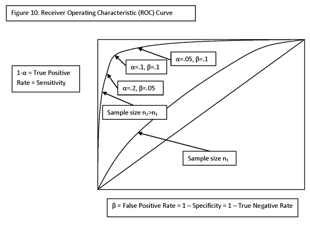
A TEST OF HYPOTHESIS WILL CORRESPOND TO A POINT ON THE ROC CURVE, I.E., TO A PARTICULAR CHOICE FOR α AND β. WHAT VALUES ARE SELECTED FOR α AND β WILL DEPEND ON THE RELATIVE IMPORTANCE OF THE TYPE I AND TYPE II ERRORS. IT IS IMPORTANT TO CONSIDER THE TRADE-OFF BETWEEN α AND β, AND NOT BLINDLY ACCEPT A STANDARD VALUE FOR EITHER.

5. MORE COMPLEX ESTIMATORS: ADJUSTMENT FOR COVARIATES; CONTINUOUS TREATMENT VARIABLE; MULTIPLE TREATMENT LEVELS

ADJUSTMENT FOR COVARIATES

IN THE PRECEDING DISCUSSION, THE ESTIMATORS WERE SIMPLE DESIGN-BASED ESTIMATORS INVOLVING MEANS AND DIFFERENCES OF MEANS FOR BINARY TREATMENT VARIABLES (E.G., “TREATED” AND “UNTREATED”). THESE ESTIMATORS ARISE IN EXPERIMENTAL DESIGNS INVOLVING RANDOMIZED ASSIGNMENT TO TREATMENT. IN MANY APPLICATIONS, FULL RANDOMIZED ASSIGNMENT IS NOT FEASIBLE, AND IT IS NECESSARY TO USE MORE COMPLEX ESTIMATORS, THAT TAKE INTO ACCOUNT EXPLANATORY VARIABLES (COVARIATES) THAT MAY AFFECT OUTCOME OR SELECTION FOR TREATMENT.

OTHER VARIABLES ARE TAKEN INTO ACCOUNT BY MAKING USE OF A STATISTICAL MODEL THAT DESCRIBES THE RELATIONSHIP OF OUTCOME (OR SELECTION FOR TREATMENT) TO THESE VARIABLES (AS WELL AS TO TREATMENT). DESCRIPTIVE SURVEYS (FOR MONITORING) ARE CONCERNED SIMPLY WITH DESCRIPTION OF POPULATION OR SUBPOPULATION CHARACTERISTICS OR EMPIRICAL RELATIONSHIPS. ANALYTICAL SURVEYS (FOR EVALUATION) ARE CONCERNED WITH ATTRIBUTION OF CAUSAL EFFECTS (SUCH AS TREATMENT), AND THE STATISTICAL MODEL USED IS DERIVED FROM A CAUSAL MODEL. THE CAUSAL MODEL IS BASED ON BELIEFS ABOUT CAUSAL RELATIONSHIPS AND ANALYSIS OF THEM (SEE Judea Pearl, Causality: Modeling, Reasoning, and Inference, 2^nd ed., Cambridge University Press, 2009 (1^st ed. 2000) FOR METHODOLOGY OF CAUSAL MODELING). SEE Jeffrey M. Wooldridge, Econometric Analysis of Cross Section and Panel Data, 2nd ed., The MIT Press, 2010, or William H. Greene, Econometric Analysis, 7th ed., Prentice Hall, 2012 FOR METHODOLOGY OF CAUSAL ANALYSIS.)

A STANDARD APPROACH TO ADDRESSING COVARIATES IS THE GENERAL LINEAR STATISTICAL MODEL. THIS MODEL MAY BE IMPLEMENTED (ANALYZED, PRESENTED) EITHER AS A MULTIPLE REGRESSION ANALYSIS OR AN ANALYSIS OF COVARIANCE. THE ANALYSIS OF COVARIANCE FRAMEWORK IS USEFUL FOR HIGHLY STRUCTURED, BALANCED DESIGNS AND FOR MULTIPLE TREATMENT LEVELS AND TREATMENT VARIABLES. IT WAS MUCH-USED IN THE ERA BEFORE COMPUTERS (WHEN INVERSION OF LARGE MATRICES WAS IMPRACTICAL, AND EXPERIMENTAL DESIGNS WERE CONSTRUCTED TO FACILITATE MANUAL ANALYSIS), BUT TODAY IT HAS BEEN LARGELY REPLACED BY THE GENERAL-LINEAR-MODEL FRAMEWORK. IT IS STILL USED FOR INSTRUCTIONAL PURPOSES AND TO SUMMARIZE HIGHLY STRUCTURED DESIGNS. THAT FRAMEWORK WORKS WELL FOR THE EXAMPLES PRESENTED HERE.

THE GENERAL LINEAR MODEL IS USEFUL FOR CONTINUOUS OUTCOME VARIABLES. FOR DISCRETE OUTCOME VARIABLES, THE GENERALIZED LINEAR MODEL (INVOLVING A GENERAL LINEAR MODEL FOR A FUNCTION OF THE MEAN) IS USEFUL. THE GENERALIZED LINEAR MODEL WILL NOT BE DISCUSSED HERE.

IN THE EXAMPLES WE CONSIDER, FOR A SINGLE BINARY TREATMENT VARIABLE THE EFFECT OF PRIMARY INTEREST IS EITHER THE COEFFICIENT OF A MAIN EFFECT (E.G., A TREATMENT EFFECT, IN THE CASE IN WHICH THE EFFECT OF INTEREST IS A SINGLE DIFFERENCE IN MEANS) OR OF AN INTERACTION EFFECT (E.G., A TREATMENT X TIME INTERACTION EFFECT, IN THE CASE IN WHICH THE EFFECT OF INTEREST IS A DOUBLE-DIFFERENCE IN MEANS).

IN THE CASE OF A BINARY TREATMENT VARIABLE, A REGRESSION COEFFICIENT REPRESENTING THE TREATMENT EFFECT IS SIMILAR TO (OR EQUAL TO) A DIFFERENCE (OR DOUBLE DIFFERENCE) OF GROUP MEANS, AND USEFUL SAMPLE-SIZE ESTIMATES CAN USUALLY BE OBTAINED BY THE METHODS ALREADY DESCRIBED (INVOLVING DESIGN-BASED ESTIMATORS). FOR PRELIMINARY ESTIMATION OF SAMPLE SIZE, A REASONABLE APPROACH IS TO APPROXIMATE A MORE COMPLEX ESTIMATOR BY ONE OF THE SIMPLER DESIGN-BASED ESTIMATORS ALREADY CONSIDERED, AND USE THE SAMPLE SIZE ASSOCIATED WITH THE SIMPLER ESTIMATOR.

IN OTHER WORDS, ALTHOUGH THE ANALYSIS INVOLVES USE OF A REGRESSION MODEL, THE EX ANTE SAMPLE-SIZE ESTIMATION MAY BE DONE IN THE USUAL FASHION, IGNORING THE MORE COMPLICATED MODEL THAT WILL BE USED IN THE DATA ANALYSIS.

A POSSIBLE EXCEPTION TO THIS GENERAL APPROACH IS THE SITUATION IN WHICH CONSIDERABLE INFORMATION IS ARE AVAILABLE ABOUT THE RELATIONSHIPS TO BE STUDIED, AND IT IS EXPECTED THAT THE PRECISION OF THE ESTIMATE OF IMPACT WILL BE SUBSTANTIALLY INCREASED WHEN THE COVARIATES ARE TAKEN INTO ACCOUNT (IN WHICH THE SAMPLE SIZE REQUIRED TO ACHIEVE A SPECIFIED LEVEL OF POWER IS REDUCED). SUCH A SITUATION IS UNUSUAL FOR EX ANTE ESTIMATION OF SAMPLE SIZE.

A SECOND EXCEPTION TO THE GENERAL APPROACH CONCERNS EX POST OR POST HOC POWER ANALYSIS. AFTER THE DATA ARE COLLECTED AND ANALYZED, THE POWER OF A TEST FOR DETECTING AN EFFECT OF THE OBSERVED SIZE MAY BE ESTIMATED. THIS USE OF STATISTICAL POWER ANALYSIS IS CALLED EX POST OR POST HOC POWER ANALYSIS. EX POST POWER ANALYSIS USES MUCH MORE COMPLEX MODELS THAN EX ANTE POWER ANALYSIS – THEY ARE THE MODELS DERIVED FROM THE DATA ANALYSIS. THIS PRESENTATION DOES NOT ADDRESS EX POST POWER ANALYSIS. FOR MORE INFORMATION ON THIS TOPIC, SEE Design and Analysis of Group-Randomized Trials by David M. Murray (Oxford University Press, 1998). ADDITIONAL REFERENCES ON POWER ANALYSIS AND THE GENERAL LINEAR MODEL INCLUDE: Statistical Methods for Rates and Proportions by Joseph Fleiss (Wiley, 1973); Linear Models by Shayle R. Searle (Wiley, 1971); Variance Components by Shayle R. Searle, George Casella and Charles E. McCulloch (Wiley, 1992); Linear Statistical Inference and Its Applications 2^nd ed. By C. Radhakrishna Rao (Wiley, 1965, 1973); Generalized, Linear and Mixed Models by Charles E. McCulloch, Shayle R. Searle and John M. Neuhaus (Wiley, 2008); and Linear Models for Unbalanced Data by Shayle R. Searle (Wiley, 1987).

ALTHOUGH THIS PRESENTATION DOES NOT ADDRESS EX POST STATISTICAL POWER ANALYSIS, TWO EXAMPLES OF SUCH ANALYSIS ARE PRESENTED. THESE EXAMPLES, CONDUCTED BY THE AUTHOR, ARE EXTRACTED FROM REPORTS IN THE PUBLIC DOMAIN. THE REPORTS DOCUMENT WORK DONE FOR THE MILLENNIUM CHALLENGE CORPORATION (MCC).

1. Final Report (Revised), Impact Evaluation of the Farmer Training and Development Activity in Honduras, NORC at the University of Chicago (Chicago, IL and Bethesda, MD), Millennium Challenge Corporation, Washington, DC, November 26, 2013.

2. Final Report (Revised), Impact Evaluation of the Transportation Project in Honduras, NORC at the University of Chicago (Chicago, IL and Bethesda, MD), Millennium Challenge Corporation, Washington, DC, December 20, 2013.

EXAMPLE 1, FROM THE REPORT, IMPACT EVALUATION OF THE FARMER TRAINING AND DEVELOPMENT ACTIVITY IN HONDURAS, NOVEMBER 26, 2013:

Ex Post Statistical Power Analysis

One of the issues to address with respect to the estimated impacts is whether the small number of statistically significant results is an indication of low power. That is, to address whether the sample size may not be sufficiently large to detect effects of anticipated or realized size. Statistical power analysis was done at the beginning of the project to estimate sample size (see Annex 3). That ex ante power analysis was complicated by the fact that the standard error of the impact estimates was not known (at that time, prior to the survey). For that reason, the power analysis was based on a model that involved a number of parameters about the test, the population under study, and the sample design. Now that the data analysis has been completed, estimates are available for the standard errors of the impact estimates, and an ex post (or post hoc) power analysis may be conducted much more easily than the ex-ante power analysis. It depends on just the test parameters (significance level; test direction (one-sided or two-sided)) and the standard error of the impact estimate. The significance level, α, of the test is the probability of a Type I error of making a decision that the effect (impact) is present (different from zero) when it is not. The probability of a Type II error of making a decision that the effect is not present when it is, is β. The power is 1 – β.

There are a number of indicators that may be examined in an ex post power analysis. Two standard indicators are the power of the test to detect a true effect equal in magnitude to the observed effect, and the minimum detectable effect (MDE) that can be detected for a specified level of power, which we shall set at 90%. The formula for the first indicator is:

for a two-sided test and

for a one-sided test, where denotes the impact estimator and denotes the standard error of this estimate. (The power formulas and notation presented here are from David M. Murray, Design and Analysis of Group-Randomized Trials, Oxford University Press, 1998.)

The formula for the second indicator is:

for a two-sided test, where α = .05 and β = 1 – power = .1, and

for a one-sided test.

For α = .05 and β = .1, the critical t values are

Two other indicators of interest in an ex post power analysis are the power to detect an effect equal to 10 percent of the mean of an outcome variable of interest and the power to detect an effect equal to 10 percent of the standard deviation of an outcome variable of interest. These are standard cases often considered in ex ante power analysis, and it is of interest to estimate the power for these two cases after the data have been analyzed and values are known for the various parameters that were unknown at the beginning of the study. The power is calculated for these two indicators from the same formula given above (for the first indicator), simply by substituting the effect size (ten percent of the mean or standard deviation) in place of .

It is also of interest to calculate the ratio of the standard error of the estimate to the mean and to the standard deviation. These indicators are related to the two just described. The latter one is of interest for estimating the (Kish) design effect of the study.

The following table presents the indicators just described, for a selection of the outcome variables, for primary roads. The table is constructed using one-sided tests, in which case, for α = .05 and β= .1 the value of t_critical:α + t_critical:β = 1.6449 + 1.2816 = 2.9265.

The power to detect an effect equal in magnitude to the observed effect is shown in column 4 of the table. This indicator is of interest only for the larger effects, since if a true effect is small, the power to detect it will be, too. The minimum detectable effect for a test of power 90% is shown in column 5. The most interesting indicators are shown in columns 9-14 – the power to detect effects equal in magnitude to various percentages of the variable (base year) mean and standard deviation.

The sample size for the evaluation was determined by statistical power analysis, i.e., by determining the sample size required to achieve a specified level of power for detecting an effect (impact, measured by the double difference measure) of specified size. When this evaluation project began, it was represented that the program intervention could easily double the income of a rural farmer, from that provided by raising traditional crops (basic grains). The initial power calculations were based on this assumption. As time passed, the assessment of program impact grew more conservative, and the sample size was estimated to achieve high power for detecting impacts equal to .5, .33, and .25 of the baseline income. As mentioned, the M&E Plan estimated an economic rate of return of 36% for the FTDA project.

The table that follows shows the power of the sample size used in the evaluation to detect impacts equal to 1.0, .5 and .25 of the base year mean, for selected outcome variables. For most outcome variables, the power to detect impacts of these magnitudes is very high. The evaluation was not “underpowered.” The power to detect impacts of the size anticipated was very high.

A revealing indicator of the power of the design is the ratio of the standard error of the estimated impact to the variable mean. This is shown in the penultimate column of the table. For an effect to be statistically significant, it has to be about twice as large as the entry in this column, as a fraction of the mean. This means that for some of the outcome variables (the smaller components of income), impacts would have to be a substantial proportion of the mean, in order to detect them with high power. (For example, the relative standard error of the estimate of impact for NetHHInc is .124. Twice this is .248. This means that for the impact of NetHHInc to be statistically significant, the effect would have to be about 25 per cent of the mean NetHHInc. This is in line with the minimum detectable effects specified at the beginning of the project (e.g., an ERR of 36%). This magnitude change may be expected for some of the indicators, but this magnitude change would not be expected for all indicators. As another example, the relative standard error of IncOC is .225. Twice this is .45. In the planning phase of the study, it was represented that the program could produce changes of this magnitude.

The last column is useful for estimating the design effect of the study. For estimation of double differences, the standard deviation of the double difference estimator if simple random sampling is used for all four design groups (if of equal size) is 4σ/sqrt(n), where σ denotes the standard deviation and n denotes the total sample size for all four groups. The value of the design effect is deff = (standard error of estimate) / (4σ/sqrt(n)) = (sqrt(n)/4) (standard error of estimate) / (Round 0 sd). From the last column, it is seen that the average value (over the outcome variables) of the ratio of the standard error of the estimate to the Round 0 standard deviation is about .08. The value of n is 7262, so deff is approximately equal to .08 sqrt(7262)/4 = 1.70. This value of deff is in line with what was expected for the design (e.g., for an intra-unit (aldea) correlation coefficient of icc = .1 and a within-unit household sample size of m = 20, deff = 1 + (m-1)icc = 2.9; for icc= .03 and m=20, we obtain deff = 1 + (20-1).03 = 1.57).

The table includes a column that specifies the coefficient of variation (CV) of the outcome variables for Round 0. The coefficient of variation is the standard deviation divided by the mean. It is presented in the column headed “CV (sd/mean)” in the table. In the power calculations done at the beginning of the project, not much was known about the statistical properties of the population with respect to the variables of interest. Data were available from which the CV for income could be estimated, and it was seen to be in the range 1-2. The sample data show that the CV is often much larger than this.

Table A.13. Intra-unit correlation coefficients for sampling units of various sizes
IncEmp	.324	.025
IncEmpAg	.311	.027
IncEmpNonAg	.427	.045
TotHHExp	.465	.069
NetHHInc	.347	.021	.040	.033	.048
CostToSchool	0	.013
TimeToSchool	.462	.109
CostToCollege	0	0
TimeToCollege	.524	.27449
CostToHospital	.020	.053
TimeToHospital	.639	.215
CostToHealthCtr	.355	.020
TimeToHealthCtr	.523	.228
CostToMarket	.254	.027	.053	.100	.083
TimeToMarket	.619	.318	.217	.262	.323
CostToPulp	0	.010
TimeToPulp	.288	.067
TimeToTegus	.861	.188
TimeToSPS	.810	.316
TimeToDepCap	.382	.162
TimeToMunCap	.366	.362
ChldInSch712	.544	.012	.012	.020	.027
ChldInSch1318	.397	.007
VisHospital	.199	.002
VisPrHlthCtr	.132	.012
VisPubClinic	.154	.013	.009	.018	.033
VisNonProf	0	.007
VisPharm	.012	.003
WrkdPrevWk	.470	.007	.007	.011	.007

Table A.17. Ex Post Statistical Power Analysis of Ordinary-Least-Squares (OLS) Regression Estimate of Average Treatment Effect (ATE) based on Continuous Treatment Variables, for Selected Outcome Measures
*Household Income and Expenditure*
IncEmp	5.00	41.5	.066	121.	4632	6033	1.30	.999+	.999+	.001	.008	.0090	.00688
IncEmpAg	71.9*	17.9	.991	52.	753	2218	2.95	.993	.999+	.095	.032	.0237	.00807
IncEmpNonAg	-109*	30.1	.976	88.	3779	5058	1.34	.999+	.999+	-.029	-.022	.0080	.00595
TotHHExp	-25.2	23.0	.292	67.	5245	4066	.78	.999+	.999+	-.005	-.006	.0044	.00566
NetHHInc	422	609	.172	1782.	77052	89246	1.16	.999+	.999+	.005	.005	.0079	.00682
*Access*
CostToSchool	-.0232	.0228	.266	.0667	.12	1.70	14.17	.212	.328	-.193	-.014	.1900	.0134
TimeToSchool	-.119	.0718	.505	.210	14.3	13.56	.95	.999+	.999+	-.008	-.009	.0050	.00529
CostToCollege	-.424	.361	.319	1.056	10.0	63.81	6.38	.870	.999+	-.042	-.007	.0360	.00566
TimeToCollege	-.180	.212	.214	.620	53.3	44.56	.84	.999+	.999+	-.003	-.004	.0040	.00476
CostToHospital	-3.52*	.718	.999	2.101	52.0	96.78	1.86	.999+	.999+	-.068	-.036	.0138	.00742
TimeToHospital	.704*	.263	.849	.770	112.	65.08	.58	.999+	.999+	.006	.011	.0023	.00404
CostToHealthCtr	-.194*	.097	.639	.284	5.39	16.49	3.06	.999+	.999+	-.036	-.012	.0180	.00588
TimeToHealthCtr	-.549*	.168	.947	.492	43.5	36.52	.84	.999+	.999+	-.013	-.015	.0039	.00460
CostToMarket	-.606*	.239	.813	.699	25.2	36.77	1.46	.999+	.999+	-.024	-.016	.0095	.00650
TimeToMarket	-.083	.240	.098	.702	82.2	58.53	.71	.999+	.999+	-.001	-.001	.0029	.00410
CostToPulp	-.126*	.0613	.659	.179	.28	5.85	20.89	.999+	.999+	-.450	-.022	.2189	.0105
TimeToPulp	-.0394	.0704	.140	206	7.91	12.01	1.52	.999+	.999+	-.005	-.003	.0089	.00586
TimeToTegus	-1.38*	.476	.894	1.39	241.	137.6	.57	.999+	.999+	-.006	-.010	.0020	.00346
TimeToSPS	.757	.994	.189	2.91	269.	159.3	.59	.999+	.999+	.003	.005	.0037	.00624
TimeToDepCap	-.459	.557	.206	1.63	112.	67.89	.61	.999+	.999+	-.004	-.007	.0050	.00820
TimeToMunCap	-1.106*	.387	.886	1.074	68.8	53.96	.78	.999+	.999+	0.016	-.020	.0056	.00717
*School Attendance*
ChldInSch712	-.00402	.00470	.216	.0138	.874	.997	1.14	.999+	.999+	-.004	-.004	.0054	.00471
ChldInSch1318	-.000843	.00375	.081	.0110	.371	.666	1.80	.999+	.999+	-.023	-.001	.0101	.00563
*Use of Health Care Services*
VisHospital	.00675	.00700	.248	.020	.306	1.11	3.63	.999+	.999+	.022	.006	.0228	.00631
VisPrHlthCtr	.00230	.00621	.101	.018	.303	.977	3.22	.999+	.999+	.076	.002	.0205	.00636
VisPubClinic	-.0513	.01058	.999	.031	.64	1.55	2.42	.999+	.999+	-.080	-.033	.0165	.00683
VisNonProf	-.0255	.00722	.969	.021	.222	1.29	5.81	.999+	.999+	-.115	-.020	.0325	.00560
VisPharm	-.00702	.00479	.429	.014	.13	.631	4.85	.993	.999+	-.054	-.011	.0368	.00759
*Employment*
WrkdPrevWk	.00436	.00649	.166	.0190	1.80	1.23	.68	.999+	.999+	.002	.004	.0036	.00528

Comparing the impact effect sizes to the means and standard deviations of the variables (in the Round 0 summary tables presented earlier), the magnitudes of the observed effects (impacts) are seen to be very small. The evaluation design was able to detect these very small effects in the response variables. For many outcome variables, the standard error of the estimate is less than one percent of the variable mean, and yet the impact is statistically significant.

While the power of the CTV estimates is high, there is a disturbing fact that emerges from Table A.17. This is the fact that the power is high because the CTV model was able to detect very small effects – on the order of one percent of the means and standard deviations of outcome variables – not because the effects are large. This high power owes to use of the GIS-model travel times (which estimates the travel-time change under the assumption that all project road improvements are completed and maintained). The estimation of sample size that was done at the beginning of the project assumed that minimum detectable effects (MDEs) would be in the range of 10-20% of the standard deviation of selected outcome variables (or of the mean, for variables with coefficient of variation approximately equal to one). That size MDE was considered because that was the magnitude of the impacts that was considered by the MCC Compact Monitoring and Evaluation (M&E) Plan for other indicators (for example, an Economic Rate of Return (ERR) of 17-21% for the primary-road improvements and at least 12-15% for rural roads). For many of the income variables, the magnitudes of the impacts that resulted from the road improvement projects were substantially less than ten percent (of the mean or of the standard deviation). Had it turned out that the impact evaluation models been able to detect MDEs of on the order of 10-20 percent, as planned, few statistically significant results would have been observed. The study would have been underpowered. The reason why the evaluation was in fact able to detect impacts of the small size that were realized was because of the very high power of the model when it incorporated the traffic survey / GIS-model information, and estimated impacts conditional on completion and maintenance of all planned road improvements. The implication of these results is that if a roads-improvement evaluation is planned, the second round of the evaluation survey should be conducted after sufficient time has elapsed for the economic benefits to manifest, and the improved roads should be maintained.

Summary of Ex Post Statistical Power Analysis

Based on this ex post statistical power analysis, it is concluded that the power of the evaluation design was quite adequate to detect effects of the anticipated size, and is reasonably characterized as high. The reason for the high power for the CTV estimates is the fact that they are conditional on GIS-model travel-time estimates, which are based on the assumption that all planned road improvements were completed and maintained.

A major recommendation for future road improvement evaluations is that if they are to be based solely on household survey data (and not traffic surveys/‌GIS-model travel-time estimates) and evaluated before the results of the project have had a chance to manifest fully, then the sample sizes must be much larger than the sample sizes used in this evaluation. Alternatively, and more reasonably, the evaluation should be delayed until the economic benefits of the project have had time to manifest. Since improvements to rural roads do not last unless the roads maintained, there is little point to evaluating such projects if they are not maintained.

As was noted in the discussion of the BTV-based estimates, the estimated effects (impacts) of the Transportation Project and the FTDA Project are confounded (because the projects were conducted in some of the same areas over the same time). Because the CTV model is based on the GIS travel-time model (and not simply on a double difference, as was the case for the BTV model), it is believed that the degree of confounding is low.

THE APPROACH TO SAMPLE-SIZE ESTIMATION WHEN COVARIATES ARE INVOLVED IS THE SAME AS BEFORE. SUPPOSE THAT THE ESTIMATE OF INTEREST IS A REGRESSION COEFFICIENT. A SAMPLE-SIZE ESTIMATE IS OBTAINED BY DETERMINING THE VARIANCE OF THE REGRESSION COEFFICIENT (INVOLVING A FACTOR OF 1/n, SAY vif/n), AND THEN SOLVING FOR n, AS DONE EARLIER. A PROBLEM THAT ARISES IN MANY APPLICATIONS IS THAT THE FORMULA FOR THE VARIANCE DEPENDS ON SO MANY PARAMETERS AND IS SO COMPLEX THAT, EX ANTE, LITTLE CAN BE SAID ABOUT IT. FROM A PRACTICAL VIEWPOINT, SAMPLE-SIZE ESTIMATION IS RARELY BASED ON COMPLEX MODELS.

THE EXTENT TO WHICH DESIGN PARAMETERS OCCUR IN THE MODEL VARIES FROM A “MODEL-ASSISTED” CASE IN WHICH MANY OR ALL OF THE DESIGN PARAMETERS ARE INCLUDED TO A “MODEL-BASED” OR “MODEL-DEPENDENT” CASE IN WHICH FEW OR NONE OF THE DESIGN PARAMETERS ARE PRESENT.

WHEN COVARIATES ARE ADDED TO A MODEL, THE DESIGN PARAMETERS MAY BECOME LESS IMPORTANT. FOR EXAMPLE, CONSIDER AN AGRICULTURAL STUDY INVOLVING A TWO-STAGE DESIGN IN WHICH A FIRST-STAGE SAMPLE OF VILLAGES IS SELECTED AND A SECOND-STAGE SAMPLE OF HOUSEHOLDS IS SELECTED FROM EACH SAMPLE VILLAGE. SUPPOSE THAT AN IMPORTANT OUTCOME OF INTEREST DEPENDS STRONGLY ON PRECIPITATION, TEMPERATURE, ELEVATION AND VEGETABLE PRODUCTIVITY INDEX, WHICH ARE AVAILABLE PRIOR TO THE SURVEY FROM A GEOGRAPHIC-INFORMATION-SYSTEM DATA SOURCE. IF THESE EXPLANATORY VARIABLES ARE NOT INCLUDED IN THE MODEL, THE “VILLAGE” EFFECT MAY BE VERY IMPORTANT, BUT IF THEY ARE INCLUDED, IT MAY BE RELATIVELY UNIMPORTANT.

THE FOLLOWING WILL PRESENT TWO VERY SIMPLE EXAMPLES OF SAMPLE-SIZE ESTIMATION FOR MODELS INVOLVING COVARIATES. EVEN THESE SIMPLE EXAMPLES SHOW THAT EX ANTE POWER ANALYSIS INVOLVING MODELS THAT CONTAIN COVARIATES IS NOT PRACTICAL.

THE EXAMPLES THAT FOLLOW ARE FOR INFORMATION / REFERENCE ONLY. THEY ARE NOT DISCUSSED IN THE ORAL PRESENTATION.

EXAMPLE: TWO DESIGN GROUPS, SIMPLE RANDOM SAMPLING, WITH AND WITHOUT COVARIATES

Suppose that the regression model that describes the relationship of the outcome (response) to design parameters and covariates is, for an individual observation:

y = x’β + ε

where y is the outcome variable, β is a (column) vector of parameters (regression coefficients), x’ is a (row) vector of explanatory variables and ε is an error term. The first explanatory variable is the mean, the second is the (binary) treatment variable and the remaining explanatory variables are the covariates. More will be said about the model error term, ε.

The preceding model represents a single observation (and y, x and ε are usually indexed with subscript i). For the complete sample, the model equation is:

y = Xβ + ε

where y is the vector of the outcome variable (y’ = (y₁, y₂,…, y_n), where n denotes the number of observations), X is the model matrix (data matrix, design matrix, incidence matrix) consisting of all of the x’s, and ε is the vector of error terms.

If all of the explanatory variables were fixed effects, then it may often be assumed that the error terms are uncorrelated with constant variance, σ². Then the (co)variance matrix of y is var(y) = σ²I (where I is the diagonal matrix having all 1’s in the diagonal). The least-squares estimate of the regression coefficients in that case is b = (X’X)^-1X’y, and the variance of the estimate, b, is var(b) = (X’X)^-1 σ².

The problem that arises with covariate analysis is that the covariates are usually considered to be random variables, each with its own variance. This is the case even for descriptive surveys, when all of the “design” variables are fixed. In this case, the preceding formulas for the estimated coefficients and their standard errors do not apply (the estimate is still unbiased, but it may be inefficient (i.e., of lower precision than is possible), and the variance formula is not correct).

In this case, the preceding model equation may be written as

y = Xβ + Zu + ε,

where the β denotes all of the fixed effects with model matrix X and u denotes the random effects with model matrix Z, ε denotes a vector of error terms ε = y –E(y|u). The random effects have mean zero and variance matrix var(u). The variance matrix of y is V = var(y) = var(Zu + ε) = Z var(u) Z’ + σ_ε²I. The best linear unbiased estimate (“BLUE”) of any linear function λ’Xβ of the fixed effects is λ’X(X’V^-1X)^-X’V^-1y (where the superscript -1 denotes inverse and superscript “^–“ denotes generalized inverse), with variance λ’X(X’V^-1X)^-X’λ.

In the preceding model, in an experimental design with randomized assignment of units to treatment, the covariates are uncorrelated with the treatment effect. In a quasi-experimental design or analysis of observational data, the lack of randomized assignment to treatment usually introduces correlations between the treatment indicator variable and the covariates.

A difficulty that arises here is that the estimate involves the variances of the covariates, which are typically unknown. To address this problem, these variances must be estimated along with the other model parameters. There are many parameters, and the estimation equations are complicated, so that numerical methods are required for solution. A procedure for doing this is the EM (Estimation-Maximization) algorithm.

Note that application of the usual “bootstrap” method for estimating variances of estimates of interest works only if the resampling is properly applied to all random variables in the model – it does not work if it is applied as if the sample design were simple random sampling. Even if applied correctly, however, that method does not involve a formula for the variance as a function of sample size, and so it is of no use for ex ante sample-size estimation. If the model is sufficiently complicated that numerical methods are required to estimate the variance of the estimator of interest, that model is of no use for ex ante estimation of sample size.

From the viewpoint of ex ante estimation of sample size, using models that involve covariates is not useful. In general, the expression for the variance is not a simple function of n and a small number of design parameters (which can be solved for n, the sample size).

Having stated the position that estimation of sample size is in general not feasible using models based on covariates, we shall present two examples to illustrate this point. The examples will include a treatment variable and group randomization (cluster randomization), with and without covariates. We present results first for the case in which there are no covariates, and then present the case with covariates. We consider the case of an experimental design in which treatment is randomly assigned to clusters. In this case, the treatment indicator variable is a fixed effect. Even this simple example illustrates the difficulties associated with estimation of sample size for models that include covariates.

The examples will be presented in two (general linear model) analysis formats – first, analysis of variance, and then, regression analysis.

Analysis-of-variance model with group randomization, excluding covariates

The following examples are similar to those presented in Murray op. cit.

In the case of cluster sampling (group randomization), the model equation is:

y_i:j:k = μ + T_k + G_j:k + ε_i:j:k

where the colon (:) is read “in”, y_i:j:k denotes the i-th observation in group (cluster) j under treatment k, μ denotes the grand mean, T_k denotes the treatment effect (the treatment is applied to all units in the j-th cluster), G_j:k denotes the effect of the j-th group under treatment k, and ε_i:j:k denotes a model error term. In this model, groups are nested within treatment, and individual observations are nested within groups. It is assumed that there are t=2 treatment levels (categories), g groups within each treatment level, and m members within each group.

The analysis of variance table for this model is as follows:

An advantage of the analysis of variance table is that it clearly shows a test of the hypothesis of equality of treatment means: the ratio of MS_t to MS_g:t is a non-central F distribution, which has a central F distribution under the hypothesis of equality of the treatment means.

In this application, there are just two treatment levels (treatment and control), so t = 2. (In this case, the square root of the ratio just mentioned obeys a Student’s t distribution.) The standard error of a difference, Δ, in means for the treatment variable is given by

at this point, we have presented two different formulas for the variance of the treatment effect, δ. The first one was based on the formula for an estimated difference using cluster sampling:

where ρ is the intra-cluster correlation

The second one is the formula for a difference in treatment means based on the estimated variance of treatment means from the analysis of variance table. The variance of the treatment means is provided by the mean square that has the same variance components as the means square for treatment, except for the component associated with treatment:

The last expression follows from the next-to-last since

σ_y² = σ_e² + σ_g²

σ_e² = ρ σ_y²

σ_g² = (1-ρ) σ_y².

Hence we see that the two different expressions for the variance of the estimator are equivalent.

Regression-model representation (excluding covariates)

The preceding model representation is used for analysis of variance, but for regression analysis the model is described with a separate parameter for each degree of freedom:

y_i = β₀ + β₁t + Σ_ju_jx_j + ε_i

where y_i denotes the i-th observation, t denotes the treatment indicator variable (t = 0 for control, t=1 for treatment), x_j denotes the indicator variable for the j-th cluster (=1 if the observation is in the j-th group (cluster), 0 otherwise), β₀ denotes the mean, β₁ denotes the treatment effect and u_j denotes the effect of the j-cluster. For simplicity, we omit one of the clusters, so that the model is of full rank. The u’s and ε’s have zero mean and are uncorrelated. The variance of u_j is σ₁² and the variance of ε_i is σ₂².

The variance of y_i (dropping the subscript) is (since t is fixed and since for each observation only one x is equal to 1 and all of the others are zero)

var(y|t) = σ₁² + σ₂².

We shall denote the total variation in y, including the variation associated with treatment, as

σ_y² = E(var(y|t)) + var(E(y|t)) = σ₁² + σ₂² + (μ₁ –μ₂)²/2.

The estimate of impact is the second regression coefficient (the coefficient of the binary treatment variable). In general, the variance of this estimate is a function of all of the estimated coefficients. While that case may arise in the data analysis, it is not illuminating for purposes of sample-size estimation. For sample-size estimation, it is necessary to consider a simpler example. As mentioned, in an experimental design involving random assignment to treatment, the covariates are independent of treatment, and that is the case we consider here.

In this case, if the clusters were considered fixed, the variance of the second regression coefficient would be

where n is the total sample size (for both groups), x denotes the 0-1 treatment indicator variable (1 for treatment, 0 for control), p is the proportion of observations assigned to treatment, σ_y² is the variance of y (i.e., the total variance about the grand mean, prior to consideration of any model (except for a mean)) and R² is the coefficient of determination of the regression model (square of the multiple correlation coefficient). For p = .5 (treatment and control samples of the same size), p(1-p) = ¼, and the above expression is 4(1-R²)σ_y²/n = 4(1-R²)σ_y²/mgt = 2(1-R²)σ_y²/mg, since n = mgt and t=2 in this example.

The problem that arises is that, in evaluation problems, the clusters are random, not fixed. Despite this situation, the preceding expression has been presented, incorrectly, as the variance of b₂ in analytical surveys for evaluation. That error overestimates power and underestimates the sample size required to achieve a specified level of power.

The correct expression for the variance is obtained from the general expression for the variance of a linear function in a general linear model, or from the analysis of variance table presented above, which is:

Since

this expression may be written as

This expression contrasts with the expression

which resulted when the variation in the clusters was ignored.

A second problem with this formulation is that the regression model includes the treatment variable, and, prior to the survey, the relationship of outcome to treatment is not known – determining that relation is a purpose of the survey.

Analysis-of-variance model with group randomization, including covariates

The model is the same as given above, with the addition of a covariate:

y_i:jh:k = μ + T_k + G_j:k + S_h + TS_kh + GS_jh:k + ε_i:jh:k

where S_h denotes the covariate. In this example, the covariate has a discrete number of levels (s) – the covariate is a variable of (post)stratification. The analysis of variance table for this model is as follows:

In this model, the effect of the intervention is represented in the TS interaction term. From the table, it is seen that a test of the equality of treatment means is provided by the ratio MS_ts/MS_gs:t.

The standard error of a difference, Δ, in means for the treatment variable is given by

It is of interest to observe how the preceding variance changes as the sample size is increased, and after the covariate is added to the model. For simple random sampling, the variance decreases in inverse proportion to the sample size n=mgt. For cluster sampling, the variance decreases inversely with mg. When the covariate is (or covariates are) added, the variance of the residual error decreases by the ratio (1 – R_adj²)/(1 – R_unadj²) (since the residual error variance is (1 – R²)σ_y²). The effect on the residual error variance, however, has little to do with the effect on the variance of the estimate of interest (Δ). The reason for this is that the effect of the covariate may differ for the various components of variance.

The relationship is as follows:

where

and

THE PROBLEM THAT ARISES WITH THIS FORMULATION IS THAT, PRIOR TO CONDUCTING THE SURVEY, WE DO NOT KNOW MUCH ABOUT THE RELATIONSHIP OF OUTCOME TO TREATMENT OR TO THE COMPONENTS OF VARIANCE (GROUPS OR COVARIATES) – THAT IS THE REASON FOR CONDUCTING THE SURVEY. WHILE THIS (REGRESSION-MODEL) APPROACH MAY BE REASONABLE FOR EX POST POWER ANALYSIS (TO DETERMINE THE POWER ASSOCIATED WITH OBSERVED EFFECTS, AFTER THE DATA ANALYSIS AND MODEL CONSTRUCTION HAS BEEN COMPLETED), IT IS NOT VERY USEFUL FOR EX ANTE POWER ANALYSIS AND ESTIMATION OF SAMPLE SIZE.

THE SAMPLE-SIZE ESTIMATION FORMULAS PRESENTED EARLIER WERE GIVEN IN TERMS OF THE VARIANCE OF y CONDITIONAL ON TREATMENT. IT IS REASONABLE TO EXPECT THAT SOME IDEA ABOUT THIS VALUE WOULD BE AVAILABLE PRIOR TO THE SURVEY, WHILE IT IS NOT REASONABLE TO EXPECT THAT INFORMATION WOULD BE AVAILABLE ABOUT THE REGRESSION MODEL, EITHER BASED SOLELY ON TREATMENT OR ON TREATMENT PLUS COVARIATES. FOR THIS REASON, THE REGRESSION MODELS DISCUSSED IN THIS SECTION ARE USEFUL MAINLY FOR EX POST POWER ANALYSIS, NOT FOR PRELIMINARY ESTIMATION OF SAMPLE SIZE.

THE PRECEDING EXAMPLES HAVE DEALT WITH ESTIMATION OF A SINGLE DIFFERENCE IN MEANS. FOR A DOUBLE-DIFFERENCE, THE APPROACH IS SIMILAR, BUT THE ANALYSIS OF VARIANCE TABLE IS LONGER (I.E., INCLUDES A TIME (SURVEY ROUND, PANEL) VARIABLE). THE TREATMENT EFFECT WOULD BE AN INTERACTION OF TREATMENT AND TIME.

THE PRECEDING APPROACH DEALT WITH POWER ANALYSIS FOR POSTSTRATIFICATION. THE APPROACH AND CONCLUSIONS ARE SIMILAR FOR MODELS INVOLVING OTHER TYPES OF COVARIATES AND MATCHING.

THE PRECEDING ILLUSTRATED THE CASE FOR A BINARY TREATMENT VARIABLE. THE ANALYSIS OF VARIANCE APPROACH IS ALSO APPLICABLE FOR MULTIPLE TREATMENT LEVELS, FOR HIGHLY STRUCTURED DESIGNS.

THE PRECEDING EXAMPLES WERE BASED ON THE GENERAL LINEAR MODEL. THE SITUATION FOR A GENERALIZED LINEAR MODEL (E.G., A LOGISTIC REGRESSION, OR A TWO-STEP MODEL) IS EVEN MORE COMPLICATED.

THE POINT TO THE PRECEDING EXAMPLES IS THAT MODELS INVOLVING COVARIATES AND MORE COMPLEX MODELS (E.G., MULTIPLE TREATMENT LEVELS, MULTIPLE TREATMENT VARIABLES, GENERALIZED LINEAR MODELS, TWO-STEP ESTIMATORS, MATCHING ESTIMATORS, TIME-SERIES INTERVENTION ANALYSIS MODELS) ARE, IN GENERAL, NOT APPROPRIATE FOR USE IN EX ANTE ESTIMATION OF SAMPLE SIZE.

6. OTHER APPROACHES

THE APPROACH PRESENTED HERE FOR ESTIMATION OF SAMPLE SIZE FOCUSES ON CONSIDERATION OF A NUMBER OF STANDARD ESTIMATORS AND DESIGNS, IN CASES IN WHICH THE SAMPLE SIZE (INCLUDING THE CLUSTER SAMPLE SIZE) IS SUFFICIENTLY LARGE THAT “LARGE SAMPLE” THEORY CAN BE USED TO DEVELOP SAMPLE-SIZE ESTIMATION FORMULAS.

REFERENCES ON THE USE OF STATISTICAL POWER ANALYSIS, BOTH FOR EX POST POWER ANALYSIS AND FOR EX ANTE ESTIMATION OF SAMPLE SIZE FOR EXPERIMENTS AND SURVEYS, INCLUDE THE FOLLOWING:

Murray, David M., Design and Analysis of Group-Randomized Trials, Oxford University Press, 1998. This text provides a thorough (detailed and comprehensive) of statistical power analysis for group-randomized (cluster-randomized) designs.

Spybrook, Jessaca, Howard Bloom, Richard Congdon, Carolyn Hill, Andres Martinez, and Stephen Raudenbush, Optimal Design Plus Empirical Evidence: Documentation for the “Optimal Design” Software, Applies to Optimal Design Plus Version 3.0, Last Revised October 16, 2011, William T. Grant Foundation. Posted (with software) at Internet William T. Grant Foundation website http://www.wtgrantfoundation.org/resources/consultation-service-and-optimal-design . This software performs statistical power analysis for a variety of person-randomized or group-randomized (cluster-randomized) experimental designs. The software allows for blocking and covariates, but does not account for stratification or matching, assumes fixed-effect covariates, and fits polynomials to describe change over time. These restrictions notwithstanding, the software distills the many model parameters into a small set which the software user may vary to explore power and sample size over a wide range of conditions. The authors of the software indicate that the methodology is intended for use in randomized designs.

Bloom, Howard S., ed., Learning More from Social Experiments: Evolving Analytic Approaches, an MDRC Project, Russell Sage Foundation, 2005.This book describes power analysis for a variety of designs, similar to (but not as extensive as) the Optimal Design software (on which Bloom later collaborated).

Bloom, Howard S., “Sample Design for Group-Randomized Trials,” PowerPoint presentation posted at Internet web site http://www.ipr.northwestern.edu/qcenter/stage/727_2_bloom/ClusterSampleDesign.ppt .

Sullivan, Kevin M., Sampling for Epidemiologists, posted on Internet web site http://www.sph.emory.edu/~cdckms/ (“Kevin’s Web Page”) at http://www.thehnts.org/useruploads/files/sampling7n.pdf . From the document: “This document describes how to calculate proportions with confidence intervals assuming simple random sampling (SRS), one-stage cluster surveys (1sc), probability proportional to size (PPS) cluster sampling, and stratified cluster sampling. Sample size calculations are also presented.” The designs do not include matching or covariates, or pretest-posttest designs.

Fleiss, Joseph L., Statistical Methods for Rates and Proportions, Wiley, 1973. Contains much information on statistical power analysis and sample-size determination for analysis of categorical data, using simple random sampling. See also Alan Agresti, Categorical Data Analysis (Wiley, 1990) and Alan Agresti, An Introduction to Categorical Data Analysis (Wiley, 1996) for additional discussion.

Pearson, E. S. and H. O. Hartley, Biometrika Tables for Statisticians, Vols. I (3^rd ed. 1966) and II (1^st ed., 1976), Biometrika Trust. These tables (Table 10 in Vol. 1 and Tables 27-30 in Vol. 2) are for fixed-effects models and simple random sampling, so they are not very useful for most evaluation settings (which involve more complex designs and random effects).

Kuehl, Robert O., Design of Experiments: Statistical Principles of Research Design and Analysis, 2^ndedition, Brooks/Cole, 2000. Kuehl presents power tables (similar to the Biometrika tables) for use with both fixed-effects and random-effects analysis of variance. The latter (random effects) are useful for power analysis in evaluation applications involving small sample sizes.

Cohen, Jacob, Statistical Power Analysis for the Behavioral Sciences, 2^nd ed., Lawrence Erlbaum Associates, 1988 (first edition Academic Press 1969). This book presents power estimates for a number of situations, but the analysis of variance and regression models assume fixed effects, so they are of little interest for evaluation applications.

Maxwell, Scott E., “Sample Size and Regression Analysis,” Psychological Methods 2000, Vol. 5, No. 4, pp. 434-458. Presents guidance on sample size for constructing large regression models from observational data. The article discusses power analysis for estimation of regression coefficients in models having a substantial number of explanatory variables. For a designed experiment or quasi-experimental design, or when differencing is applied to the data, the number of explanatory variables is usually small. This methodology applies more to analysis of observational data than to experimental design or quasi-experimental design.

THE REFERENCES THAT ARE RESTRICTED TO SIMPLE RANDOM SAMPLING ARE NOT OF DIRECT RELEVANCE TO THE SAMPLE SURVEY DESIGN OR EVALUATION DESIGN. THESE SOURCES DO NOT MAKE THE “LARGE SAMPLE” ASSUMPTION, AND SO THE METHODOLOGY IS MORE COMPLICATED (INVOLVING NONCENTRAL t AND F DISTRIBUTIONS INSTEAD OF THE STANDARD NORMAL (z) DISTRIBUTION USED HERE). THESE REFERENCES CONSIDER THE CASE OF MULTIPLE TREATMENT LEVELS (HENCE THE F DISTRIBUTION), WHEREAS THE PRESENTATION HERE HAS FOCUSED ON A BINARY TREATMENT VARIABLE (TREATMENT VS. CONTROL).

7. COMPUTER SOFTWARE

COMPUTER SOFTWARE FOR IMPLEMENTING THE APPROACH TO SAMPLE SIZE DETERMINATION PRESENTED HERE IS POSTED AT INTERNET WEB SITE http://foundationwebsite.org (under the title “Computer program for determining sample size). HERE FOLLOWS SAMPLE OUTPUT FOR THE PROGRAM, FOR THE CASE OF ESTIMATING SAMPLE SIZE TO ACHIEVE A SPECIFIED LEVEL OF POWER FOR ESTIMATING A DOUBLE DIFFERENCE MEASURE.

EXAMPLE OF OUTPUT FROM COMPUTER PROGRAM

Figure 11a. Example of Output from Sample-Size Computer Program, page 1

Figure 11b. Example of Output from Sample-Size Computer Program, page 2

FndID(213)

FndTitle(SAMPLE SIZE ESTIMATION FOR MONITORING AND EVALUATION: LECTURE NOTES)

FndDescription(SAMPLE SIZE ESTIMATION FOR MONITORING AND EVALUATION: LECTURE NOTES)

FndKeywords(sample size; sample size estimation; sample size determination; statistical precision analysis; statistical power analysis)

*Table A.16. Ex Post* Statistical Power Analysis for Selected Impact Estimates**
Outcome Variable	Estimate of Impact (observed effect)	Standard error (se) of estimate	Power of test to detect a true effect equal in magnitude to the estimate of impact	Minimum detectable effect (MDE) for a test of power 90%	Round 0 mean	Round 0 standard deviation (sd)	CV (sd/mean)	Power to detect a true effect equal to 1.0 of Round 0 mean	Power to detect a true effect equal to 1.0 of Round 0 sd	Power to detect a true effect equal to .5 of Round 0 mean	Power to detect a true effect equal to .5 of Round 0 sd	Power to detect a true effect equal .25 of Round 0 mean	Power to detect a true effect equal to .25 of Round 0 sd	Std error of estimate relative to Round 0 mean	Std error of estimate relative to Round 0 std dev
IncBG	-120	837	.070	2450	7682	14017	1.82	1.0	1.0	.997	1.0	.742	.993	.109	.0600
ExpBG	837	393	.686	1150	2991	5350	1.79	1.0	1.0	.983	1.0	.602	.959	.131	.0735
NetBG	-957	750	.356	2195	4691	10966	2.34	1.0	1.0	.928	1.0	.468	.977	.160	.0684
LabExpBG	351	264	.376	773	931	2924	3.14	.969	1.0	.547	1.0	.223	.868	.284	.0903
IncOC	16773	4298	.987	12578	19103	65316	3.42	.996	1.0	.718	1.0	.297	.983	.225	.0658
ExpOC	5413	1078	.999	3155	4532	13650	3.01	.993	1.0	.676	1.0	.277	.933	.238	,0788
NetOC	11360	4175	.858	12218	14571	56737	3.89	.996	1.0	.540	1.0	.221	.959	.287	.0736
LabExpOC	1911	742	.823	2171	1878	8360	4.45	.811	1.0	.350	1.0	.156	.878	.395	.0888
IncEmp	149	733	.078	2145	6450	9851	1.53	1.0	1.0	.995	1.0	.710	.956	.114	.0744
TotHHExp	204	496	.110	1452	5375	4922	.916	1.0	1.0	1.0	1.0	.856	.798	.092	.1008
NetHHInc	18926	13306	.412	38940	107379	157043	1.46	1.0	1.0	.991	.903	.645	.903	.124	.0847
Horticulture	-.0397	.0194	.656	.0568	1.9227	.2670	.139	1.0	1.0	1.0	1.0	1.0	.962	.010	.0727

Table A.17. Intra-unit correlation coefficients for sampling units of various sizes
Outcome Variable	Sampling unit (level of sampling in multistage sampling)
Outcome Variable	Household	*Aldea*	Municipality	Department
IncBG	.475	.033	.016	.044
ExpBG	.461	.027	.016	.051
NetBG	.348	.031	.020	.029
LabExpBG	.223	.013	.017	.027
IncOC	.486	.042	.026	.054
ExpOC	.404	.029	.028	.059
NetOC	.433	.045	.022	.046
LabExpOC	.267	.022	.022	.030
IncEmp	.423	.033	.026	.024
TotHHExp	.272	.040	.066	.040
NetHHInc	.504	.040	.025	.028
Horticulture	.051	.007	.029	.032

Table A.12: Ex Post Statistical Power Analysis for Selected Impact Estimates Based on Binary Treatment Variables, for Primary Roads
Outcome Variable	Estimate of Impact (observed effect)	Standard error (se) of estimate	Power of test to detect a true effect equal in magnitude to the estimate of impact	Minimum detectable effect (MDE) for a test of power 90%	Round 0 mean	Round 0 standard deviation (sd)	Power to detect a true effect equal to .1 of Round 0 mean	Power to detect a true effect equal to .1 of Round 0 sd	Estimate of impact relative to Round 0 mean	Estimate of impact relative to Round 0 sd	Standard error of estimate relative to Round 0 mean	Standard error of estimate relative to Round 0 standard deviation
IncEmp	689.	448.	.457	1311.	4632.	6033	.277	.391	.148	.114	.0967	.0743
IncEmpAg	-101.	194.	.132	568.	753.	2218	.106	.312	-.134	-.040	.2576	.0875
IncEmpNonAg	849.*	327.	.828	957.	3779.	5058	.319	.471	.235	.168	.0865	.0647
TotHHExp	180.	249.	.179	729.	5245.	4066	.687	.503	.034	.044	.0475	.0672
NetHHInc	6836.	6574.	.274	19239.	77052.	89246	.325	.395	.089	.077	.0853	.0737
TimeToSchool	-.317	.776	.110	2.27	14.28	13.56	.589	.552	-.022	-.023	.0543	.0574
TimeToMarket	-2.35	2.60	.231	9.61	82.17	58.53	.950	.757	-.029	-.040	.0316	.0444
ChldInSch712	.114*	.0509	.723	.149	.874	.997	.529	.623	.130	.114	.0582	.0511
VisPubClinic	-.220*	.115	.606	.337	.64	1.55	.142	.397	-.344	-.142	.1797	.0742
WrkdPrevWk	.0846	.0705	.329	.206	1.80	1.23	.817	.540	.047	,069	.0392	.0573

Table A.13. Intra-unit correlation coefficients for sampling units of various sizes
Variable	Sampling unit (level of sampling in multistage sampling)
Variable	Household	Caserío	Aldea	Municipality	Department
IncEmp	.324	.025
IncEmpAg	.311	.027
IncEmpNonAg	.427	.045
TotHHExp	.465	.069
NetHHInc	.347	.021	.040	.033	.048
CostToSchool	0	.013
TimeToSchool	.462	.109
CostToCollege	0	0
TimeToCollege	.524	.27449
CostToHospital	.020	.053
TimeToHospital	.639	.215
CostToHealthCtr	.355	.020
TimeToHealthCtr	.523	.228
CostToMarket	.254	.027	.053	.100	.083
TimeToMarket	.619	.318	.217	.262	.323
CostToPulp	0	.010
TimeToPulp	.288	.067
TimeToTegus	.861	.188
TimeToSPS	.810	.316
TimeToDepCap	.382	.162
TimeToMunCap	.366	.362
ChldInSch712	.544	.012	.012	.020	.027
ChldInSch1318	.397	.007
VisHospital	.199	.002
VisPrHlthCtr	.132	.012
VisPubClinic	.154	.013	.009	.018	.033
VisNonProf	0	.007
VisPharm	.012	.003
WrkdPrevWk	.470	.007	.007	.011	.007

SAMPLE SIZE ESTIMATION FOR MONITORING AND EVALUATION: LECTURE NOTES

1. APPROACH TO SAMPLE SIZE ESTIMATION

2. SAMPLE SURVEYS FOR MONITORING AND EVALUATION -OVERVIEW

3. SAMPLE SIZE ESTIMATION FOR DESCRIPTIVE SURVEYS

4. SAMPLE SIZE ESTIMATION FOR ANALYTICAL SURVEYS

5. MORE COMPLEX ESTIMATORS: ADJUSTMENT FOR COVARIATES; CONTINUOUS TREATMENT VARIABLE; MULTIPLE TREATMENT LEVELS

Intra-unit correlation coefficients

6. OTHER APPROACHES

7. COMPUTER SOFTWARE