Optimal Attack and
Defense for a Number of Targets in the Case of Imperfect Interceptors
This
article describes the optimal defense of a set of targets against an optimal
attack, in the case of imperfect interceptors. This solution is obtained from
a mathematical representation of strategic nuclear warfare as a two-sided
resource-constrained optimization problem. The attacker and defender are
assumed to know each other's total force sizes, and it is assumed that the
attacker "moves last," i.e., the attacker allocates his weapons to
targets after observing the defender's allocation of interceptors to targets.
A one-on-one (or fixed salvo-to-one) firing doctrine is assumed. The
attacker's goal is to maximize the total damage to the targets, and the
defender's goal is to minimize this damage. It is assumed that damage on any
single target can be adequately described by the "exponential" damage
function defined below.
Let
us denote the total number of weapons by X and the total number of interceptors
by Y. Further, let us denote the number of targets by t, and the number of
weapons and interceptors allocated to the i-th target by xi and yi,
respectively. The attacker's and defender's strategies are hence specified by
vectors
x' = (x1, x2,..., xt)
and
y' = (y1, y2,..., yt)
where
each xi > 0, yi > 0, and
Σ(i:1,t) xi = X
and
Σ(i:1,t) yi = Y
where
the notation Σ(i:1,t) denotes the summation operator over the index i, ranging
from 1 to t.
Using
the exponential damage function, the expected damage at the i-th target is
Di(zi) = Pi(1
- exp(-βizi))
where
zi is the number of weapons reaching the i-th target, Pi
is the value of the i-th target, and βi is the damage function
parameter for the i-th target.
The
interceptor kill probability, κ, is assumed to be the same for all targets.
The
attacker is assumed to choose his strategy x after observing the
strategy y selected by the defender. He will choose a strategy x*(y)
such that
H(x*(y*),y) = max(x)
H(x,y),
where
H(x,y) denotes the total expected damage corresponding to the
strategies x and y, and max(x) denotes maximization with
respect to x (of the following function of x, in this case H(x,y)).
The defender hence must choose his strategy y* such that
H(x*(y*),y*) = min(y)
max(x) H(x,y) ,
and
min(y) denotes minimization with respect to y.
Using
the exponential damage function, the expected damage on the i-th target is
shown in Appendix A to be PiQi where
1 - exp(-αixi) ,
xi < yi
Qi =
1 - exp(-βi(xi-yi))
exp(-αiyi) , xi > yi ,
and
αi < βi is defined by the equation
exp(-αi) = (1 - κ)exp(-βi)
+ κ .
The
total expected damage is
H(x,y) = Σ(i:1,t) Hi(xi,yi)
= Σ(i:1,t) PiQi
.
We
shall denote the expected damage corresponding to the optimal solutions x*,
y* as H(X,Y).
Our
problem, thus, is to determine x*,y* such that
H(x*,y*) = min(y) max(x)
H(x,y)
where
H(x,y) = Σ(i:1,t) PiQi
subject
to the constraints
Σ(i:1,t) xi = X
Σ(i:1,t) yi = Y
and
xi > 0, yi > 0. The function H(x,y)
is additively separable over the targets so the Everett-Pugh double Lagrange
multiplier technique (References 2 and 3) can be used to find a solution. The
problem becomes one of finding xi, yi corresponding to
min(yi) max(xi) (PiQi
- λxi + μyi)
where
λ, μ are adjusted so that the constraints
Σ(i:1,t) xi = X
and
Σ(i:1,t) yi = Y
are
satisfied. If there are several choices of (μ,λ) for which the constraints can
be met (i.e., there are several solutions to the double Lagrange multiplier
problem), the correct optimal solution to the problem is the solution
corresponding the least damage.
For
convenience we drop the subscript i, so that the problem is to find x, y
corresponding to
min(y) max(x) (PQ - λx + μy) .
The
solution is derived in Appendix A (Technical Details). The next section will describe
the results.
The
solution to the above two-sided optimization problem is complicated to describe
analytically, and can be described best in geometrical terms. Appendix A
contains such a description. In this section we shall present only a
qualitative description of the optimal attack and defense allocations.
Note
that the mathematical approach used to solve the present problem assumes that
the xi's and yi's are continuous variables, rather than
integers. This approximation introduces a negligible error whenever the number
of interceptors and weapons allocated to targets are zero or large enough that
the fractional parts are insignificant.
The
optimal solution can conveniently be described by observing how the weapon and
interceptor allocations to targets change for a fixed total defense level, Y,
as we very the total offense level, X, from zero to a very large number. In
all situations, weapons are allocated to targets so that the marginal payoff
per weapon is the same on all targets. Note that for a specified X, there may
be some targets that, even if undefended, yield so little payoff to the
attacker that they are not attacked. Such targets are not defended, either.
For a specified total defense level, Y, there are two total attack levels, Xmin(Y)
and Xmax(Y), that are of special significance. We shall describe
the nature of the solution in terms of these levels.
When
the attack level is less than the value Xmin(Y), every attacked
target is defended by a number of interceptors that exceeds the number of
weapons assigned to it. Thus damage to targets can occur only through
"leakage", i.e., failure of the interceptors to kill all incoming
weapons. The defense allocation is arbitrary, so long as there are more
interceptors than weapons on each attacked target. The attack allocation for
specified X is unique. The total payoff to the attacker is an increasing
concave ("diminishing returns") function of the total attack level,
X.
For
all attack levels lying between the values Xmin(Y) and Xmax(Y),
the defense is unique. Such a defense is called "stable." In this
region of attack levels, the attacker can choose between two different attack
levels on each target. The lower level may be zero on some targets. The
attacker must attack each target at either the lower level or the higher level,
and can choose to attack at any combination of these permissible levels that
meets his total attack level, X. The payoff is a linear function of the total
attack level in this region.
The
situation in the case of the low and intermediate attack levels is referred to
as "defense dominant".
As
the total number of weapons is increased above the level Xmax(Y),
the defender must change his allocation. He does so by defending fewer
targets, but defending the defended targets at a higher level. As the attack
size increases, eventually only one target would be attacked. Also, for a
sufficiently large attack size all targets would be attacked. Since the
defense allocation changes as the attack size changes in this region, the
defense is called "unstable". Both the attack and defense
allocations corresponding to specified X are unique.
The
situation in the case of a high attack level is called "attack
dominant".
The
solutions to the present problem are derived by the method of generalized
Lagrange multipliers. Using this technique, we can find a solution for every
total attack level X < Xmin(Y). Over the range Xmin(Y)
< X < Xmax(Y), however, there are only a finite
number of Lagrangian solutions, corresponding to all possible combinations of
low level or high level attacks on each attacked target. For a large number of
weapons, interceptors, and targets, there is a very large number of such
solutions, and there would be a Lagrangian solution corresponding to a total
attack size quite close to any specified total attack level. Hence in practice
we need only concern ourselves with the Lagrangian solutions. (Solutions
corresponding to other total attack levels differ very little from Lagrangian
solutions corresponding to nearby total attack levels. These other solutions
are less "efficient" than the Lagrangian solutions, since the payoff
function for them lies below the marginal payoff for the additional weapons
used (beyond those required by the closest Lagrangian solution using fewer weapons)
is less than the total marginal payoff achieved by going to the next higher
Lagrangian solution. This latter marginal payoff is defined by the slope of
linear payoff function defined by the Lagrangian solutions.)
Over
the range X > Xmax(Y), there can be found a Lagrangian solution
for any specified total attack level, X, but not for every specified total
defense level, Y. The reason for this difficulty lies with the fact that, in
the Lagrangian solution, a target can be defended at only two levels, one of
which is zero (no defense). (The situation is analogous to the intermediate
attack situation in which targets could be attacked at only two levels.) As
before, this problem is not of practical significance, since we can always find
a Lagrangian solution corresponding to a total defense level close to the
specified total defense level.
It
is of interest to compare how the nature of the solution to the allocation
problem in the case of imperfect interceptors differs from the solution in the
case of perfect interceptors. Two questions of interest are:
1. For what range of the kill probability, κ,
are the allocations and total damage essentially the same as for the perfect
interceptor case, κ = 1?
2. For specified interceptor kill probability,
κ, and total defense level, Y, is the solution to the problem
"similar" (in allocations and total damage) to the perfect
interceptor problem with total defense level κY? (Note that κY is the expected
number of interceptors that do not fail, and represents a possible
"effective" number of perfect interceptors.)
The
questions were answered by examining the nature of the solution for a
"reasonable" set of hypothetical targets, described in Table 1.
Table
1. Hypothetical Target Set
Target
Value Exponential Damage
Target Number (Population in millions) Function
Parameter (β)
1 10 .03
2 6 .04
3 4 .05
4 3 .06
5 2 .08
6 1.5 .10
7 1.0 .20
8 1.0 .30
9 1.0 .40
10 .5 .50
The
total expected damage, H(X,Y), corresponding to the optimal attack and defense
allocations is plotted in Figures 1 and 2 as a function of total attack level,
X, for fixed total defense level, Y.
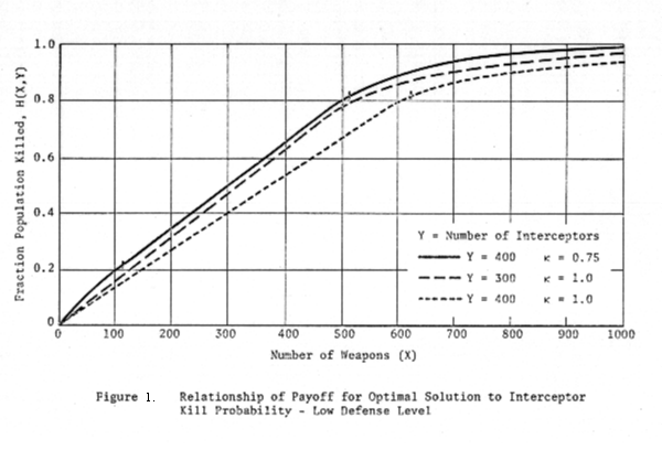
Figure
1 corresponds to Y1 = 400, and Figure 2 corresponds to Y2
= 800. On each figure are three curves:
1. H(X,Yi) for κ = 1
2. H(X,Yi) for κ = .75
3. H(X,.75Yi) for κ = 1.
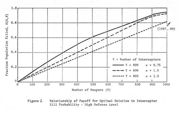
The
figures indicate first that there are substantial differences in total damage
between the κ = 1 and κ = .75 cases, and that the imperfect interceptor case is
not always closely approximated by the perfect interceptor case for total
defense level κY. However, the difference between these latter two cases is
not so great as to preclude using the "equivalent perfect
interceptor" approximation for some purposes.
This
appendix derives the optimal defense of a set of targets against an optimal
attack in the case of imperfect interceptors. It is assumed that the defender
has a total number, Y, of interceptors, and that the attacker has a total
number, X, of weapons. Let us denote the number of targets by t, and the
number of weapons and interceptors allocated to the i-th target by xi
and yi, respectively. The attacker's and defender's strategies are
hence specified by vectors
x' = (x1, x2,..., xt)
and
y' = (y1, y2,..., yt)
where
each xi > 0, yi > 0, and
Σ(i:1,t) xi = X
and
Σ(i:1,t) yi = Y .
We
assume that the exponential damage function adequately describes the expected
damage at each target; that is, the expected damage is
Di(zi) = Pi(1
- exp(-βizi))
where
zi is the number of weapons reaching the i-th target, Pi
denotes the value of the i-th target, and βi is the damage function
parameter for the i-th target.
We
assume that the attacker "moves last," i.e., he chooses his strategy,
x, after observing the strategy y selected by the defender. He
will choose a strategy x*(y) such that
H(x*(y),y) = max(x)
H(x,y)
where
H(x,y) represents the expected damage corresponding to the
strategies x and y. The defender, then, should choose his
strategy y* such that
H(x*(y*),y*) = min(y)
max(x) H(x,y) = U .
The
value U is the upper pure value of the game in which the attacker and defender
move simultaneously. Since x* and y* are pure strategies, there
is no reason why U should equal the lower pure value of such a game, defined by
L = max(x) min(y) H(x,y)
.
Both
the attacker and defender are assumed to know each other's force size and κ.
We
assume that the interceptor kill probability, κ, is the same for all targets.
The
expected damage on the i-th target if u weapons get through is given by
Di(u) = Pi(1 - exp(-βiu))
.
The
probability that u weapons get through, given that there are xi
weapons and yi interceptors, both integers, is
A if 0 < u < xi
and xi < yi
Pxiyi(u) = 0 if 0 <
u < xi-yi and xi > yi
B if xi-yi < u <
xi and xi > yi
where
A = C(xi,u)(1 - κ)u κxi
- u
and
B = C(yi,(u - (xi - yi)))
(1-κ)u - (xi - yi) κxi - u ,
and
C(n,e) denotes the combination function (i.e., the number of combinations of n
things taken e at a time). (Note: The word processing program used to display
this article cannot place subscripts or superscripts on subscripts or
superscripts; the exponents xi and yi in the preceding expressions (and in
similar expressions that follow) should be xi and yi,
respectively.)
The
expected damage on the i-th target is hence
Hi(xi,yi) =
Σ(u:0,xi) (Expected damage given that u weapons
get through) (Probability that u weapons get
through)
= Σ(u:0,xi) Pi(1 - exp(-βiu))Pxiyi(u)
= PiΣ(u:0,xi) (1 - exp(-βiu))Pxiyi(u)
= PiQi ,
where
A, xi < yi
Qi =
B, xi > yi
where
A = 1 - ((1-κ)exp(-βi)+κ)xi
and
B = 1 - exp(-βi(xi - yi))
((1 - κ)exp(-βi) + κ)yi .
We
shall use this expression for all xi, yi, not just for
integral values. We shall simplify the expression for Qi by
defining
exp(-αi) = (1 - κ)exp(-βi)
+ κ
where
αi < βi since κ < 1. Hence we have
1 - exp(-αixi)
, xi < yi
Qi =
1 - exp(-βi(xi - yi))
exp(-αiyi) , xi > yi .
The
total expected damage is
H(x,y) = Σ(i:1,t) Hi(xi,yi)
= Σ(i:1,t) PiQi .
We
shall denote the expected damage corresponding to the optimal solutions x*,
y* as H(X,Y).
Our
problem, thus, is to determine x*, y* such that
H(x*,y*) = min(y) max(x)
H(x,y)
where
H(x,y) = Σ(i:1,t) PiQi
subject
to the constraints
Σ(i:1,t) xi = X
Σ(i:1,t) yi = Y
and
xi > 0, yi > 0. Since the function
H(x,y) is not concave, the Kuhn-Tucker theorem is of no
assistance in computing the solution. The function H(x,y) is additively
separable over the targets, however, and so the Everett-Pugh double Lagrange
multiplier technique (References 2 and 3) can be used to find a solution. The
problem becomes one of finding xi, yi corresponding to
min(yi) max(xi) (PiQi
- λxi + μyi)
where
λ, μ are adjusted so that the constraints
Σ(i:1,t) xi = X
and
Σ(i:1,t) yi = Y
are
satisfied. If there are several choices of (λ,μ) for which the constraints can
be met, (i.e., there are several solutions to the double Lagrange multiplier
problem), the correct optimal solution to the problem is the solution
corresponding to the least damage. We shall for convenience drop the subscript
i; that is, the problem is to find x, y corresponding to
min(y) max(x) (PQ - λx + μy) .
The
values of the Lagrange multipliers are adjusted so that the resource
constraints are met.
The
significant feature of the generalized Lagrange multiplier (GLM) method is
that, because the damage function is additively separable (i.e., the total
damage is the sum of the damage on each target), the solution of the global
optimization problem may be found by simply solving, independently, an
unconstrained optimization problem for each target (and then adjusting the
multipliers so that the constraints are obeyed. Another reason (apart from
additive separability) why the GLM method is used in this problem is that the
damage function is not convex (so that the Kuhn-Tucker and other standard
optimization methods cannot be applied). (In addition to not requiring
convexity of the objective function, the GLM method also does not require
differentiability or continuity or linearity of the objective function.)
The
only complexity that arises in the present problem is that the two-sided GLM
procedure may produce a multiplicity of solutions for specified values of the
Lagrange multipliers, some of which may not correspond to optimal solutions.
It is hence necessary to prove that the optimal solution is contained within
the solution set, and to select it from the non-optimal solutions. (This
difficulty does not occur with the one-sided GLM method.)
The
damage function H(x,y) = PQ may be illustrated as in Figure A-1.
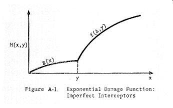
Let
us denote
g(x) = P(1 - exp(-αx))
and
f(Δ,y) = P(1 - exp(-βΔ - αy))
where
Δ = x - y > 0. Then we may write
g(x) , x < y
PQ = H(x,y) =
f(Δ,y) , x > y .
We
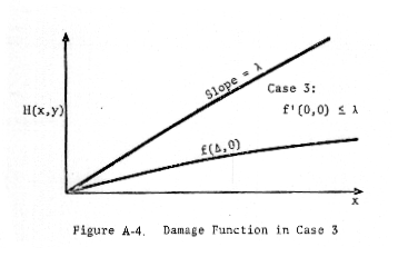
distinguish three cases:
Case 1: g'(0) < λ, f'(0,0) > λ
Case 2: g'(0) > λ (which implies f'(0,0)
> λ since α < β)
and
Case 3: f'(0,0) < λ (which implies
g'(0) < λ since α < β) ,
where
the derivative of f(Δ,y) is with respect to Δ.
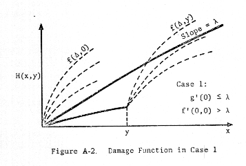
These
cases are depicted in Figures A-2, A-3, and A-4.
(The
parenthetic remarks follow since:
g(x)
= P(1 - exp(-αx)
g'(x)
= Pα exp(-αx)
g'(0)
= Pα
f(Δ,y) = P(1 - exp (-βΔ - αy)
f'(Δ,y) = Pβ exp(-βΔ - αy)
f'(0,0)
= Pβ
α < β therefore Pα < Pβ, and hence g'(0) <
f'(0,0).)
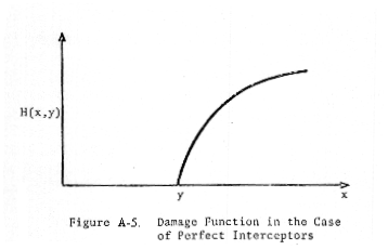
Now
Case 1 is a straightforward generalization of the problem solved by Goodrich
(pp. 12 - 19 of Reference 4). Goodrich solved this problem in the case of
perfect interceptors (κ = 1), as depicted in Figure A-5.
The
solution in Case 1 is as follows. For specified y, consider the line passing
through the origin and tangent to the damage curve (see Figure A-6). (Note:
The Figure A-6 does not clearly show that the damage curve has slope lower than
the tangent line at the origin.)
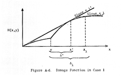
Let
us denote the slope of this line by λ'(y), the value of x at the point of tangency
by x', and denote Δ'(y) = Δ' = x' - y. Let us denote the value of x
corresponding to slope λ by xλ, and denote Δλ(y) = Δy
= xλ - y. It is easy to show (see Goodrich) that the value of x
that maximizes the Lagrangian function
L(x,y) = H(x,y) - λx + μy
is
0 if λ > λ'(y) =
λ'
x* =
xλ if λ < λ'(y) = λ'
(either
value, 0 or xλ, may be chosen if λ = λ'). Denoting Δ'(y) = Δ' = x'
- y, we have that
f'(Δ',y) == λ' = f(Δ',y)/(Δ' + y) ,
(where
the differentiation is with respect to Δ and the double equal sign, ==, denotes
"is identically equal to") and we may rewrite the optimal x-solution
as
0 if λ > f(Δ',y)/(Δ'
+ y)
x* =
xλ = Δλ + y if λ <
f(Δ',y)/(Δ' + y) .
Note
that if f'(0,0) < λ (Case 3), then x* = 0, for then (since f'(Δ,y) <
f'(0,0) < λ) there is no point x such that f'(Δ,y) = λ, regardless of the
value of y). (This follows by the following:
f'(Δ,y) = Pβ exp(-βΔ - αy)
f'(0,0)
=-Pβ
f'(Δ,y) = Pβ exp(-βΔ - αy) < f'(0,0) (since
exp(-βΔ - αy) < 1)
so
if f'(0,0) < λ then f'(Δ,y) < λ for all x,y, so that
there are no roots if f'(0,0) < λ.)
Substituting
the above solution x* into L(x,y), we obtain
μy if λ
> f(Δ',y)/(Δ'+y)
L(x*,y) =
f(Δλ,y) - λ(Δλ+y) + μy if
λ < f(Δ',y)/(Δ'+y) .
Note
that we have substituted Δλ + y for xλ in the above,
because we wish to represent y explicitly. We wish to choose y to minimize
L(x*,y).
It
is interesting, but not necessary for the solution, to note that f(Δλ,y)
depends only on λ, in the case of the exponential damage function. We will now
demonstrate this. Now Δλ is defined by the equation
f'(Δλ,y) = λ
where
the differentiation of f(Δ,y) is with respect to Δ. Note that Δλ
depends on y. Since
f(Δ,y) = P(1 - exp(-βΔ - αy)) ,
we
have
f'(Δ,y) = Pβexp(-βΔ - αy) ,
so
that
Pβexp(-βΔλ - αy) = λ ,
so
that
f(Δλ,y) = P(1 - λ/Pβ) ,
which
depends only on λ. Hence we could write
f(Δλ,y) = f(λ)
in
the case of the exponential damage function.
This
result is interesting, since if implies that the damage is the attacker's
(heavier) optimal attack corresponding to the value λ is the same (for the
exponential damage function), whether the defender chooses to defend the target
or not (since the height of the damage function is the same (f(Δλ,0)
= f(Δλ,y)) in either case). (If, in the optimal attack against a
defended target, the attacker has two attack options (e.g., 0 and xλ),
the no-defense damage (optimal attack) is the same as the damage at the heavier
optimal attack level against the defended target.) We observe from the
expression for f(λ) that the fraction surviving the optimal attack is λ/Pβ.)
Continuing
with the (general) solution, we observe that we can write the Lagrangian
function as
μy
if λ > f(Δ',y)/(Δ' + y)
L(x*,y) =
f(λ) - λ(Δλ + y) + μy if λ <
f(Δ',y)/(Δ' + y)
μy if y > f(Δ',y)/λ - Δ'
=
f(λ) - λ(Δλ + y) + μy if y <
f(Δ',y)/λ - Δ' .
Now
the set
S = {y │ y > f(Δ'(y),y)/λ - Δ'(y)}
= {y │ λ > f(x'+y,y)/x'}
= {y │ λ > λ'(y)} .
Now
λ'(y) = f(x'+y,y)/x' is
a monotonic increasing function of y, and so
S = {y │ y > y'}
where
y' is the unique solution to the equation
y = f(Δ'(y),y)/λ - Δ'(y) .
Hence
the Lagrangian becomes
μy if y > y'
L(x*,y) =
f(Δλ,y) - λ(Δλ+Y) + μy
if y < y' .
(For
the exponential damage function, f(Δλ(y),y) = f(λ), and y' is that y
such that
f(Δ'λ(y),y)/(y + Δ'λ(y)) = λ
i.e.,
f(λ)/(y' + Δ'λ(y')) = λ
f(λ)/ λ = y' + Δ'λ (y')
y'
= f(λ)/λ - Δ'λ(y') .)
Since
L(x*,y) is hence a piecewise linear function of y, the value of y that
minimizes L(x*,y) occurs either as y = 0 or at the solution y = y' to the
equation
y = f(Δ'(y),y)/λ - Δ'(y) .
Substituting
these values into L(x*,y), we obtain
L(x*,0) = f(Δλ(0),0) - λΔλ(0)
and
L(x*,y') = μy'
= (μ/λ)(f(Δ'(y'),y') - λΔ'(y')) .
To
minimize L(x*,y), we hence choose
0 if μ > λc
Y =
y' if μ < λc
where
c = (f(λ) - λΔλ(0))/(f(λ) - λΔλ(y'))
,
and
either value if μ = λc. This corresponds to the solution obtained by Goodrich
(where c = 1 in the case of perfect interceptors). (The solution represents a
"balanced defense", since the per-weapon payoff to the attacker is
the same for all targets.)
We
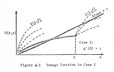
now consider Case 2, in which g'(0) > λ. (This implies f'(0,0) > λ.
Observe also that f'(0,x) > g'(x).) For specified y, consider the line
tangent to the damage function in two places, as shown in Figure A-7.
We
denote the slope of this line by λ', and the values of x at the two points of
tangency by x1' and x2'. We define x1, x2,
Δ1, Δ2, Δ1', Δ2' similarly, as
shown in Figure A-7. Since f'(0,x) > g'(x), we have x1' < y
< x2'. Since we are assuming that g'(0) > λ, the value of x
that maximizes the Lagrangian function
L(x,y) = H(x,y) - λx + μy
cannot
occur at x = 0. Rather, the optimal solution is
x1 if λ
> λ'
x* =
x2 if λ
< λ'
(either
value if λ = λ'). That this is the optimal solution follows from the
generalizated theory of Lagrange multipliers (Reference 1). Defining Δ1'
= x1' and Δ2' - x2' - y, we have
λ' == f'(Δ2',y) = (f(Δ2',y)
- g(Δ1'))/(Δ2' + y - Δ1')
(where
the differentiation is with respect to Δ2') so that we may write
x1 = Δ1
if λ > (f(Δ2',y) - g(Δ1'))/(Δ2' + y - Δ1')
x* =
x2 = Δ2 + y if λ <
(f(Δ2',y) - g(Δ1'))/(Δ2' + y - Δ1')
.
As
in Case 1, we observe that f(Δ2,y) depends only on λ in the case of
the exponential damage function. The Lagrangian function hence becomes
g(Δ1) - λΔ1 + μy
if λ > (f(λ') - g(Δ1'))/(Δ2' + y - Δ1')
L(x*,y)
=
f(λ)-λ(Δ2 + y)+μy if λ < (f(λ') -
g(Δ1'))/(Δ2' + y - Δ1')
g(Δ1) - λΔ1 + μy if
y > y'
=
f(λ) - λ(Δ2 + y) + μy if y < y'
where,
as in Case 1, we substituted Δ2 + y for x2 and where y'
is the solution to the equation
y = (f(λ) - g(Δ1λ))/λ - (Δ2λ(y)
- Δ1λ) .
Note
that L(x*,y) is continuous at y = y'. Since L(x*,y) is piecewise linear in y,
the minimum occurs either at y = 0 or at the solution y = y' to
y = (f(λ) - g(Δ1λ))/λ - (Δ2λ(y)
- Δ1λ) .
(It
is easy to show that the function L(x*,y) is always positive for y positive.)
Calculating
the value of L(x*,y) for these two values, we have
L(x*,0) = f(λ) - λΔ2(0)
and
L(x*,y) = g(Δ1) - λΔ1 +
μy'
= g(Δ1)
- λΔ1 + μ((f(λ) - g(Δ1))/λ - (Δ2(y') - Δ1)).
To
minimize L(x*,y) we hence choose y to be
0 if μ > λc
y* =
y' if μ < λc
where
c = [(f(λ) - g(Δ1))/λ - (Δ2(0)
- Δ1)] / [(f(λ) - g(Δ1))/λ - (Δ2(y') - Δ1)],
and
either value if μ = λc.
Let
us denote the attacker's optimal solution corresponding to y* by
x* = x*(y*)
0 or x' if y* = y'
=
x" if y* = 0
for
Case 1 targets, and
x1' or x2' if
y* = y'
=
x" if y* = 0
for
Case 2 targets.
Both
x* and y* are zero for Case 3 targets; that is, the only targets worth
attacking are those worth defending. Note that, since f'(x,0) > g'(x) for
small x, x" > x1' for small x1'. Further, since
f'(x - y,y) < f'(x - y,0), we have x" > x2' - y'.
An
unfortunate aspect of the solutions obtained by the double Lagrange multiplier
method is that, for specified resource levels (X and Y), there may be several
solutions, corresponding to different values of the Lagrange multipliers (μ and
λ). While all such solutions are optimal for the attacker, only one of them is
also optimal for the defender. We shall refer to this latter solution as the
"correct" optimal solution. (The others are referred to as
"spurious".) The next three sections well describe the Lagrangian
solutions in further detail, and which of them are optimal for both the
attacker and the defender simultaneously (i.e., which combinations
correspond to "correct" optimal solutions.)
We
shall now observe some properties of the attacker's optimal solutions. The
salient characteristic of the solution is that the attacker attacks each target
at a level for which the slope of damage curve is the same (λ). It is noted
that the defender either allocates no interceptors to a target, or y'
interceptors to a target, where y' is the level such that the line of slope λ
tangent to the damage curve at the attack level x > y' either passes through
the origin (in Case (1) in which g'(0) < λ), or is also tangent to the
damage curve at the attack level x < y' (in Case (2) in which g'(0) > λ).
This situation is illustrated in Figures A-8, A-9, and A-10.
(Concerning
Figure A-9: Since f'(0,x) > g'(x), there must exist Δ > 0 and y > 0
such that f'(Δ,y) = λ in this case. Note that x" > x1'
holds only if x1' is small.)
(Concerning
Figure A-10: Since f'(0,0) > g'(x), there is no x such that g'(x) = λ.)
Note
that the attacker chooses his solution after observing at each target whether
the defender defends at level 0 or y'. For reasons that will be explained
later, the attacker can attack some targets at the low level (0 for Case 1
targets and x1' for Case 2 targets) only if the defender is
defending all Case 1 and Case 2 targets at the higher level (y').
In
summary, the optimal solution for the attacker has the following properties:
1. The marginal
payoff to the attacker on all targets attacked is λ.
2. On all defended "Case 1" targets,
the ratio of damage to number of weapons is λ; on all defended
"Case 2" targets, the ratio of damage to number of weapons is greater
than λ, and this ratio is greater for the solution x1' than the
solution x2'; on all undefended Case 1 or Case 2 targets, the ratio
is greater than λ.
If
all Case 1 or Case 2 targets are defended, the total number,
Ymax(λ) == Σ yi'
where
the symbol Σ denotes summation; if all Case 1 and Case 2 targets are defended,
and attacked at the highest optimal level, the total number of weapons used is
Xmax(Ymax(λ)) == Xmax(λ)
= Σ x2i' ;
if
all Case 1 and Case 2 targets are defended, and attacked at the lowest optimal
level, the total number of weapons used is
Xmin(Ymax(λ)) == Xmin(λ)
= Σ x1i' ;
if
all Case 1 and Case 2 targets are not defended, but are attacked at the optimal
level, the total number of weapons used is
X(Y,λ)│Y=0 = X(0,λ) == Σ x3i' ;
where
we define
0 on Case 1 targets
x1i' = x1' on Case 2
targets
0
on Case 3 targets
(corresponding
to minimal attack, maximal defense);
x' on Case 1 targets
x2i' = x2' on Case 2
targets
0 on Case 3 targets
(corresponding
to maximal attack, maximal defense); and
x" on Case 1 or
Case 2 targets
x3i' =
0 on Case 3 targets
(corresponding
to an attack against no defense).
The
following characteristics of the defender's solution are noted:
1. For the complete defense, Y = Ymax(λ),
the attacker can choose not to attack any (or all) of the Case 1 targets or to
attack any of the Case 2 targets at the lower level, x1', and the
resulting deployments (attack and defense) are optimal at the new level x,
Xmin(λ) <
X < Xmax(λ) .
This characteristic results from the defender's
having chosen the defense so that the tangent at slope λ passes through the
origin (Case 1) or through both points of tangency (Case 2). The attacker is
thus indifferent to attacking at the level 0 or the level x' (Case 1), or to
attacking at the level x1' or x2' (Case 2). The damage
increases linearly (with slope λ) for all X, Xmin(λ) < X <
Xmax(λ) (this will be proved later).
2. If the defender chooses not to defend some
Case 1 or Case 2 targets, and the attacker also chooses not to attack
some defended Case 1 targets or to attack some defended Case 2 targets at the
lower level, then the resulting deployment is not optimal for the given
resource levels, X and Y, even though the deployment would be the optimal one
for the given values of λ and μ, if λ and μ represented true marginal costs of
weapons and interceptors. This paradoxical situation arises since, using the
double Lagrange multiplier method, there may be many different values of λ and
μ that correspond to the same resource levels. (See Reference 3 for a
discussion of this point). In the preceding situation, there would be a larger
value of λ that would correspond to the same total numbers of weapons and
interceptors deployed.
The
defense would prefer this latter deployment since it results in lower payoff to
the attacker. This follows since, for Xmin(λ) < X <
Xmax(λ), the payoff to the attacker is the same per weapon (beyond
the payoff of the "Xmin(λ) weapons"):
Payoff = λ(X - X0) .
For
λ1 < λ2, the payoff λ1X01 of the
"Xmin(λ1) weapons" is greater than the payoff λ2X02
of the "Xmin(λ2) weapons." Also, λ1X
< λ2X. Hence
Payoff for λ1 = λ1(X - X01)
< λ2(X - X02) = Payoff for λ2.
Hence
the defender would choose the deployment corresponding to λ2. Thus
we see that the attacker can attack on the range Xmin(λ) <
X < Xmax(λ) only if the defense is "complete"
(i.e., the defender defends at level y' in all Case 1 and Case 2 targets).
We
shall now determine which solutions are simultaneously optimal for both
the attacker and the defender.
In
the preceding section, we showed that the pair (μ,λ) corresponding to the
correct solution cannot correspond to a partial defense and a partial attack.
Rather, the correct (μ,λ) must correspond either to a complete attack, partial
defense, or to a complete defense, partial attack. We also provide that in the
complete defense case, in which Xmin(λ) < X < Xmax(λ),
if two different choices for (μ,λ) correspond to the same resource levels, the
"better" solution corresponds to the larger value of λ. In view of
the possibility of there being many different choices (μ,λ) that correspond to
the same resource levels, it is necessary to answer the following question:
How is it possible to find (μ,λ) corresponding to the solution optimal for the
specified resource levels? Our objective is twofold: (1) to make certain that
the correct (μ,λ) pair is included among all (μ,λ) pairs identified as
corresponding to the specified resource levels; (2) to test each such (μ,λ)
solution to determine if it is optimal.
In
view of the results of the preceding section, if the correct solution is
included in the set of (μ,λ) pairs identified as meeting the constraint levels,
then we will be able to select it in the complete defense case. Hence our
problem is solved for the complete defense case if we can prove that the
correct solution is among those identified.
We
can prove the correct solution is in fact included, by the following argument.
We will show that there is only one permissible choice of λ corresponding to
the complete defense case. Since the correct solution must correspond to the
complete defense case. Since the correct solution must correspond to some choice
of (μ,λ) that meets the resource constraints, and this choice is the only
permissible one, it must then be the correct solution. (There may indeed be
other values of λ which satisfy the resource constraints, but they will
correspond to partial defenses and attacks, and hence to spurious solutions.)
Note
that for values of λ greater than max(i) (Pi,βi), no
weapons and no interceptors are allocated to any target. Furthermore, as λ is
decreased to zero, the maximal number of weapons that are allocated increased monotonically
(but discontinuously) from zero. For μ > λ, no interceptors are allocated,
and for all μ < λ, the allocation is the same (all Ymax(λ)
interceptors). The upper interceptor limit increases monotonically (and
continously) as λ decreases. Hence, if we are allocating for a complete
defense, partial attack, there is only one value of λ which will meet
the defense level constraint. Hence we have the correct solution (i.e., the
solution which is simultaneously optimal for both attacker and defender) in the
complete defense case (Xmin(λ) < X < Xmax(λ)).
Note
that there may be no choice of (μ,λ) corresponding to the specified
defense and attack levels. For example, in the complete defense, minimal attack
situation, the minimal attack resource level may exceed the specified attack
resource level. In this case, we have no solution to the problem for the
specified resource levels, by the Everett-Pugh double Lagrange
multiplier technique. It is nevertheless possible to determine an optimal
solution in this case using the single Lagrange multiplier technique, by
the following reasoning. Consider the complete defense, minimal attack
situation, in which the defender defends all Case 1 and Case 2 targets, and the
attacker attacks all such targets at the minimal level (x1'). The
attacker deploys Xmin(λ) weapons in this case. If the attacker
wishes to use fewer than Xmin(λ) weapons, he must allocate his
weapons so that the marginal payoff per weapon is the same for all targets.
That is, he chooses a new value of λ, greater than λ', and chooses x' so that
g'(x') = λ'. Clearly, he will attack all targets with a number of weapons that
is less than x1', and hence less than the number of interceptors.
Since this is the case, the defender has no need to adjust his defense. He can
maintain the same defense no matter how many weapons (less than Xmin(λ))
the attacker allocates, since in every case there are fewer weapons than
defenders. Additional interceptors have absolutely no effect on the payoff.
The problem hence reduces to one of simply allocating the attacker's weapons,
using g(x) for the payoff function. Since the total number X(λ) of attackers
allocated, given λ, is a monotone decreasing function of λ. this is easily
accomplished. Note that the defense can rearrange his allocation any way he
pleases, so long as y > x on every target, and the resulting
allocation is still optimal. Only X(λ) of the interceptors are actually
needed.
Thus
we have the correct solution in the case in which X < Xmin(λ).
The
final case to consider is the complete attack case in which X > Xmax(λ).
For a specified number of defended targets, both Y(λ) and X(Y(λ),λ) increase as
λ decreases. However, there may be several different numbers of defended
targets for which λ = λ' can be chosen so that X(Y(λ'),λ') = X and Y(λ') is
close to Y. (Owing to the discrete nature of targets, it in general will not
be possible to meet the interceptor constraint exactly.) In the unlikely event
that Y(λ') is the same for two different values of λ', the better solution
corresponds to the allocation resulting in least damage. In general, however,
we will have several possible solutions, each using a different number of
interceptors and resulting in a different level of damage. The correct optimal
solution is the solution with Y(λ') < Y which has least damage. The
situation is illustrated in Figure A-11.

For
both Case 1 and Case 2 targets, the damage in the optimal attack (complete
attack case) is a function of λ only, i.e.,
Damage = f(x - y,y) = f(λ) = P(1 - λ/Pβ).
We
observe that the damage is a decreasing function of λ. Therefore, if there are
several different λ's for which the weapon constraint is met and for which the
interceptor constraint is not exceeded, then the defender will choose the
defense corresponding to the largest λ. Referring to Figure A-11, the optimal
solution is hence the rightmost one (corresponding to total resource levels X,
Y2), in which the maximum number of targets is defended.
A
useful way to summarize the several preceding observations is to plot the
payoff for optimal solutions corresponding to varying attack levels for a fixed
defense level. Such a plot is shown in Figure A-12.

Before
summarizing the nature of the solutions corresponding to the different sections
of this curve, we recall the nature of the Lagrangian solutions on the three
types of targets.
For
Case 1 targets, the defender chooses a number, y, of interceptors and the
attacker chooses a number, x, of weapons, such that the tangent line to the
damage curve at x is of slope λ, and the tangent line passes through the
origin. (See Figure A-8.) For Case 2 targets, the defender chooses y, and the
attacker chooses x2 > y, so that the tangent line to the curve at
x2 is also tangent at a point x1 < y; furthermore,
this tangent line is of slope λ. (See Figure A-9.) Case 3 targets are neither
defended nor attacked. (See Figure A-10.)
Not
all of the points described above correspond to optimal solutions. Depending
on the circumstances (to be described) the attacker may be required to attack
only at the higher level, or the defender may be required to defend only at the
higher level. We shall now describe the situation using Figure A-12, which
depicts total damage, H(X,Y) as a function of X, for fixed Y.
In
the first section of the curve, all Case 1 and Case 2 targets are defended, and
all are attacked. The defense is greater than necessary in this region, for
there are more interceptors than weapons on each target. The defense is
somewhat arbitrary here; it can be rearranged in any fashion so long as there
are always more interceptors than weapons on each target. The attack
corresponding to a specified X is unique. Both the interceptor and weapon
constraints are met exactly.
In
the second section of the curve, all Case 1 and Case 2 targets are defended,
and the defense is unique (or "stable"). The attacker may attack
each target at either the low level or the high level, and he does so in any
fashion which enables him to meet his weapon constraint, X. The interceptor
constraint, Y, is met exactly, but the weapon constraint may only be
approximated, owing to the discrete nature of weapons and interceptors. (We
refer to this error as the "small change" effect.) Thus there are
actually only a finite number of Lagrangian solutions along the linear portion
of the curve corresponding to all possible combinations of attacks at the high
or low attack levels on each target. Payoffs corresponding to total attack
levels lying between these points lie slightly below the line defined by the
payoffs of the Lagrangian solutions.
The
first two sections of the curve represent what is called a "defense
dominant" situation.
In
the third section of the curve, all Case 1 and Case 2 targets are attacked at
the higher level, but only a subset of the Case 2 targets are defended. The
defended targets have the following property. Let λ denote the value of the
(attacker's) Lagrange multiplier in the optimal attack. Suppose, now, that no
targets were defended, and that this same value of λ were used to determine the
number of weapons to be allocated to each target. Let us denote the damage to
the i-th target in such an attack by Di, and the number of weapons
by Ni. Consider the ratio Ri = Di/Ni.
If all Case 1 and Case 2 targets are arranged in decreasing order of Ri,
then the defended targets of the optimal attack are at the beginning of this
list. In other words, the defender defends targets in decreasing order of
their undefended damage per weapon.
Both
the defense and the attack are unique in this section of the curve. The weapon
constraint is met exactly, but the interceptor constraint may only be
approximated. This section of the curve represents the "attack
dominant" situation.
In
the third section of the curve, there may be several different values of λ,
corresponding to different numbers of defended targets, which enable us to meet
the weapon and interceptor constraints. The defender naturally chooses the
defense allocation which corresponds to the least damage. In the present
problem, this happens to the solution corresponding to the largest value of λ,
since in the attack dominant case the damage on the i-th target is given by
Pi(1 - λ/Piβi)
.
It
is of some interest to describe the nature of the solution as a function of the
Lagrange multiplier λ. We summarize the situation in Figure A-13 through A-17
(ignoring the "small-change" effect caused by discrete weapons and
interceptors).

Figures
A-14 and A-15 illustrate the ranges of total defense and attack levels corresponding
to optimal attacks for different values of λ.

Note
that it is not possible to obtain an optimal solution for every choice of X and
Y, by the method of double Lagrange multipliers. If Y is very large and X is
very small, there may be no value of λ for which Xmin(λ) < X and
Y < Ymax(λ). (This region is called a "gap". Regions
such as this, which are inaccessible by the Everett-Pugh procedure of
min-maxing the Lagrangian function (as opposed to zeroing its derivative, in
the case of continuously differentiable functions), represent
"inefficient" solutions. (See Reference 2 for a discussion of
gaps.) As discussed previously, however, we were able in the present problem
to find an optimal solution over this gap. (Another type of gap occurs since
the discrete nature of targets prohibits meeting both resource levels exactly.
This "small change" effect is generally small, however, for problems
involving several targets and large numbers of weapons and interceptors.)

Figure
A-16 is a plot of the payoff (denoted by H(X,Ymax(λ))) corresponding
to all possible optimal attack levels, for constant λ and Y = Ymax(λ).
(This plot is simply the middle section of Figure A-12.)

Figure
A-17 is a plot of the payoff (denoted by H(X(Y,λ),Y)) corresponding to all
possible optimal defense levels, for fixed λ.

The
plot of Figure A-17 is a level line since f(Δλ,y) = (Δλ,0), as discussed previously.
In
view of the preceding characteristics of the optimal solution, a reasonable
procedure for finding the optimal solution (corresponding to Σ xi =
X, Σ yi = Y) is the following:
1. Determine the largest value of λ such that
Ymax(λ) = Y. Compute Xmin(λ) and Xmax(λ).
2. Complete defense, partial attack case. If
Xmin(λ) < X < Xmax(λ), then the
optimal solution is obtained by attacking a sufficient number of the (Case 1 or
Case 2) targets at the higher level (x2i') to satisfy the weapon
constraint, X. (Any such collection of targets is satisfactory. This is the
case since the additional damage caused in going from x1i' to x2i'
weapons on the i-th target is λ(x2i' - x1i'). Thus the
additional damage caused by the x2i' - x1i' weapons,
above the damage caused by the x1i' weapons, is the same linear
function of the additional weapons allocated, for all targets.) Since weapons
are allocated to targets in groups, it will in general not be possible to meet
the weapon constraint exactly.
3. Complete attack, partial defense case. If
X > Xmax(λ), then decrease λ to the largest value of λ such that
Xmax(λ) = X. An optimal solution is obtained by defending a
sufficient number of the (Case 1 or Case 2) targets to satisfy the interceptor
constraint, Y. The targets to be defended must be selected in order of
decreasing ratio in the no-defense case, of damage to weapons, until Y
interceptors are used. Unfortunately, however, if some defendable targets are
not defended, then fewer weapons are allocated (see Figure A-11). Hence our
weapon constraint is not met. We must hence decrease the value of λ (giving us
new values of Ymax(λ) > Y and Xmax(λ) > X), and
choose a new set of targets to be defended. As before, we select targets to be
defended in the (new) order of decreasing ratio, in the no-defense case, of
damage to weapons, until Y interceptors are used. We compute, for this defense
allocation, the corresponding number, X(Y), of weapons. We decrease λ until
X(Y) = X. Since interceptors are allocated to targets in groups, it will in
general not be possible to meet the interceptor constraint exactly. There may,
however, be a number of different solutions (corresponding to different numbers
of defended targets) using fewer than Y interceptors, and we should choose the
one resulting in least damage (largest λ).
4. Complete attack, unnecessarily large
defense. If X < Xmin(λ), no solution can be found by the method
of double Lagrange multipliers. Either fewer than Y interceptors must be used,
or more than X weapons must be used, to obtain an optimal solution by this
method. To find the optimal solution for the specified Y, we instead use the
single Lagrange multiplier method, and proceed as follows. Accept the defense
allocation corresponding to Xmin(λ), Ymax(λ) = Y. Then,
increase the value of λ, and compute the corresponding attack allocation.
Denoting the number of weapons deployed by X(λ), adjust λ so that X = X(λ).
This allocation is the optimal attack allocation. Denoting the number of
weapons deployed by X(λ), adjust λ so that X = X(λ). This allocation is the
optimal attack allocation. Any defense allocation for which the number of
interceptors on each target exceeds the number of weapons is optimal. Hence,
in particular, the defense allocation corresponding to X = Xmin(λ),
Y = Ymax(λ), is optimal.
A
computer program has been written to perform the above computations.
The
derivation presented above of the optimal solution includes a number of
implicit relationships. The solution will now be explicitly derived.
If
f'(0,0) < λ, no weapons or interceptors are allocated to the target.
We
have
f(Δ,y) = P(1 - exp(-βΔ - αy))
so
that
f'(Δ,y) = Pβexp(-βΔ - αy)
and
f'(0,0) = Pβ .
Thus
if Pβ < λ, no weapons or interceptors are allocated to the target.
In
this case, Pβ > λ and g'(0) < λ. We have
g(x) = P(1 - exp(-αx))
so
that
g'(x) = Pαexp(-αx)
and
g'(0) = Pα .
Thus
if Pα < λ, the situation is that of Case 1. In this case, we wish
first to determine x,y > 0 such that the tangent line at the point x is of
slope λ and passes through the origin. That is, find x,y such that
f'(x - y, y) = λ
and
f(x - y,y)/x = λ .
The
first relation implies
Pβexp(-β(x - y) - αy) = λ
or
exp(-β(x - y) - αy) = λ/Pβ .
Substituting
this into the second relation, we have
P(1 - λ/Pβ)/x = λ
or
x = P(1 - λ/Pβ)/λ .
The
first relation then yields
y = (ln(λ/Pβ) + βx)/(β - α).
If
y = 0, then x must satisfy
f'(x,0) = λ
i.e.,
Pβexp(-βx) = λ
or
x = (-1/β) ln(λ/Pβ) .
Case
2 corresponds to Pα > λ (Pβ > holds since α < β). In this case, we
wish first to determine x1, x2, and y, where x1
< y < x2, such that the tangent line at the point x2
is of slope λ, the tangent line at the point x1 is of slope λ, and
these tangent lines are in fact the same line. That is, we want x1,
x2, y such that
g'(x1) = λ
f'(x2 - y,y) = λ
(f(x2 - y,y) - g(x1))/(x2
- x1) = λ.
The
first relation yields
exp(-αx1) = λ/Pα
or
x1 = -(1/α)(ln(λ/Pα)) .
The
second relation yields
exp(-β(x2 - y))exp(-αy) = λ/Pβ .
Substituting
the first two relations into the third hence yields
(P(1 - λ/Pβ) - P(1 - λ/Pα))/(x2 - x1)
= λ
or
x2 = x1 + 1/α - 1/β .
The
second relation yields
y = (ln(λ/Pβ) + βx2)/(β - α) .
In
the case in which y = 0, we wish to find x such that
f'(x,0) = λ .
As
is Case 1, we obtain
x = -(1/β)(ln(λ/Pβ)) .
1.
Hugh Everett, III, Defense Models XI: Exhaustion of Interceptor Supplies,
Lambda Paper 17, Lamdba Corporation, Arlington, Virginia, 1968. (Lambda
Corporation later became a subsidiary of General Research Corporation, McLean,
Virginia.)
2.
Hugh Everett, III, "Generalized Lagrange Multiplier Method for Solving
Problems of Optimum Allocation of Resources," Operations Research,
11:399-411, 1963.
3.
George E. Pugh, "Lagrange Multipliers and the Optimal Allocation of
Defense Resources," Operations Research, 12:543-567, 1964.
4.
Robert L. Goodrich, Defense Models V: Ivan II, A Detailed Model for Preferential
Defense, Lambda Paper 7, Lambda Corporation, Arlington, Virginia, 1968.
FndID(168)
FndTitle(Optimal
Attack and Defense for a Number of Targets in the Case of Imperfect
Interceptors)
FndDescription(This
article determines the optimal allocation of attacking missiles and defending
interceptors to targets, in the case of imperfect interceptors.)
FndKeywords(ballistic
missile warfare; ballistic missile defense; resource-constrained game; min-max
solution; generalized lagrange multipliers)