Conflict, Negotiation, and General-Sum Game Theory
Summary
To date, most war gaming, weapons allocation, and force procurement models have been developed either using zero-sum payoffs (one player's loss is the other's gain), or ignoring the relationship of conflict to negotiation. This situation prevails in spite of the fact that two-player general-sum (positive-sum) game theory has been developed to the point where both of these aspects can be taken into account. One reason for this situation is that, although good analytical solutions are theoretically determined, explicit computation of the solution is in general very difficult.
This paper examines the problem of determining a computationally tractable general-sum game-theoretic solution to war, taking into account the effect of the threat of war on negotiations. An idealized situation that seems to possess the essential characteristics of most actual situations is examined. If A and B denote the payoff matrices of the general-sum game between the players, then it is shown in general that optimal threat strategies for conducting the war are given by the optimal solutions to the zero-sum game A-cB, where the constant c is such that this game has value k (a constant depending on the nature of the particular problem). Furthermore, if all payoffs are negative, if the losses associated with combat are quite large compared to those associated with negotiation, and if the losses from negotiation are close to zero, then k is approximately equal to zero. (In addition, the optimal strategies correspond approximately to the solution of the ratio game A/B, and this game has value c.) If, further, the two players' combat losses tend to be proportional, then c is approximately equal to VA/VB, where VA and VB are the values of the zero-sum matrix games A and B. That is, approximately optimal strategies for conducting the war are given by the solutions to the zero-sum game (VB/VA)1/2 A - (VA/VB)1/2 B. Thus, the difficult mathematical problem of solving the general-sum game (which is felt to represent war more adequately than a zero-sum formulation) is reduced to a simpler mathematical problem, viz., the solving of a particular zero-sum game derived from the general-sum game.
I. Introduction
This paper will summarize current theory relating to the solution of finite two-player general-sum games, and examine certain situations which appear to relate to war and negotiation and which suggest reasonable criteria for conducting a war.
There is a well-established procedure for playing games in which the interests of the players are diametrically opposite (so that one player's loss is the other player's gain). Such a game is called a constant-sum, or zero-sum, game. For "rational" players, optimal strategies are available; these strategies are given by the minimax (von Neumann-Morgenstern) solution to the game.
A game in which the interests of the two players are not necessarily exactly opposite is called a general-sum game. The theory of general-sum games does not, in general, provide optimal strategies for the players. General-sum games are classified into two types: noncooperative and cooperative. In a noncooperative game, any type of collusion, such as side payments and correlated strategies, is not permitted between the players.
If we accept that there is a relationship between the negotiations conducted by two nations and the wars occurring between those nations, it is reasonable to view negotiation and conflict in a combined context. The interests of two nations are not in general directly opposed, i.e., it is possible for both to profit as they change their strategies. It is hence reasonable to examine negotiation and conflict as a general-sum cooperative game, in the hope of determining some useful information concerning good criteria for negotiation and waging war.
II. Background Information: Nash's Bargaining Solution to a General-Sum Game
A finite zero-sum game is characterized by a payoff (or loss) matrix, A, whose (i,j)-th element aij indicates the gain to player 1 (loss to player 2) if player 1 selects his i-th strategy and player 2 selects his j-th strategy. If, in playing the game, player 1 selects his i-th strategy with probability xi, then we say that he is employing a mixed strategy; we denote this strategy by the vector x = (x1,x2,...,xn)'. If player 1 selects strategy x and player 2 selects strategy y, then the gain to player 1 (loss to player 2) is xAy'.
If we assume that player 1 wishes to maximize his gains, and that player 2 wishes to minimize these gains (his losses), then it can be proved that there are optimal strategies, x*, y* for both players, defined by
x*Ay*' = max(x) min(y) xAy' = min(y) max(x) xAy' ,
where max(x) denotes maximization with respect to x (of the following function of x) and min(y) denotes minimization with respect to y.
A finite general-sum game is characterized by a pair of payoff (or loss) matrices, A and B. The element aij of the matrix A specifies the gain to player 1 if he selects strategy i and player 2 selects strategy j. The element bij of the matrix B specifies the gain to player 2 if player 1 selects strategy i and player 2 selects strategy j.
Unlike the situation in the constant-sum game, there is no unique "natural" solution to a general-sum game. The most reasonable approach developed to date, however, seems to be that developed by John Nash. Nash actually developed two solutions, which he calls the special bargaining solution and the general bargaining solution, respectively. We shall briefly describe these solutions. See reference 2 for further details.
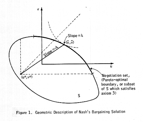
It is convenient to describe the solutions in terms of a graph showing the payoffs (u,v) accruing to the two players, corresponding to various strategies (x,y). Both solutions are defined in terms of a point (u*,v*) -- called the status quo point -- which corresponds to the least (expected) payoff that a player is willing to accept. How this point is chosen is the difference between Nash's two solutions. In general, if we do not specify the nature of the status quo point, we shall simply refer to the corresponding solution as a bargaining solution to the game.
Let us denote by S the feasible set, or set of all possible joint payoffs (u,v) realizable by the two players acting together. If A and B denote the payoff matrices of the two players, then S is the set of convex combinations of the set of points (aij,bij). Given the status quo point (u*,v*), Nash proved that if there are any points (u,v) in S, then there exists a unique point (ub,vb) (called the bargaining solution) that satisfies the following six axioms:
1. (ub,vb) ≥ (u*,v*). (That is simply a statement of the condition that neither player will accept a payoff less than u* or v*, respectively.)
2. (ub,vb) is in S.
3. If (u,v) is in S and (u,v) ≥ (ub,vb), then (u,v) = (ub,vb). (This axiom is called the condition of Pareto optimality.)
4. If (ub,vb) is in T, a subset of S, and (ub,vb) is the bargaining solution for the set S when (u*,v*) is the status quo point, then (ub,vb) is the bargaining solution for the set T with the same status quo point. (This axiom is called the condition of independence of irrelevant alternatives. It says that if both players reject feasible alternatives, then those alternatives cannot affect the solution, so long as the status quo point remains the same.)
5. The solution is linearly invariant. That is, if T is obtained from S by the linear transformation
u' = a1 u + b1
v' = a2 v + b2 ,
then, if (ub,vb) is the bargaining solution for S with status quo point (u*,v*), then (a1u + b1, a2v + b2) is the bargaining solution for T with status quo point (a1u* + b1, a2v* + b2).
6. The solution is symmetric with respect to the players. That is, if S is such that
(u,v) is in S if and only if (u,v) is in S ,
and (ub,vb) is the bargaining solution for S with status quo point (u*,v*), where u* = v*, then ub = vb.
Furthermore, Nash proved that if there are any points (u,v) in S that satisfy u > u* and v > v*, then the bargaining solution is the point (ub,vb) that maximizes the function
g(u,v) = (u - u*) (v - v*)
subject to u ≥ u* (or v ≥ v*) and (u,v) in S. (If there is no point in S such that u > u*, then u = u* for (u,v) in S, and the solution is (ub,vb) where ub = u* and
vb = max (v such that (u,v) is in S, v ≥ v*) v .
If there is no point in S such that v > v*, then v = v* for (u,v) in S, and the solution is (ub,vb) where vb = v* and
ub = max (u such that (u,v) is in S, u ≥ u*) u .)
The geometric nature of the solution is indicated in Figure 1. Note that if A and -cB are approximately equal, then the points (aij,bij) of S tend to lie on a line of slope -c, and the payoff possible through negotiation differs little from that if the players do not negotiate. If A = -cB, then we have the zero-sum situation, of course, in which negotiation is of no use (one player's loss equals the other's gain). If A is approximately equal to cB, then the points (aij,bij) of S tend to lie along the line u = cv, and there is a great deal to be gained by negotiation. If A = cB, then the interests of the players coincide, and there is but one point in the negotiation set.)
III. The Special and General Bargaining Solutions
We shall now describe how the status quo point is chosen. In the special bargaining problem, u* and v* are the payoffs that the players can obtain by unilateral action, whatever the other player does; i.e., they are the minmax values of the respective matrix games, A and B:
u* = max(x) min(y) xAy'
v* = max(y) min(x) xBy' .
Note that if A = -cB, then the general-sum game reduces to a zero-sum game.
In the general bargaining problem, u* and v* (called threat payoffs) are chosen as follows. First, we describe some characteristics of the bargaining solution. Observe from the figure that, from axiom 3, whatever the values of u* and v*, the solution (ub,vb) is restricted to that part of the boundary of S such that u and v cannot simultaneously be increased. By changing u* and v*, we move the solution (ub,vb) along the Pareto-optimal boundary, and one player can profit only if the other player loses. (This tradeoff is not linear unless the Pareto-optimal boundary is linear.) The objectives of the two players in choosing their threats (u* and v*) are directly opposed, and it can be proved that there are in fact optimal choices for u* and v*.
IV. Special Cases of Interest
A. Linear Negotiation Set
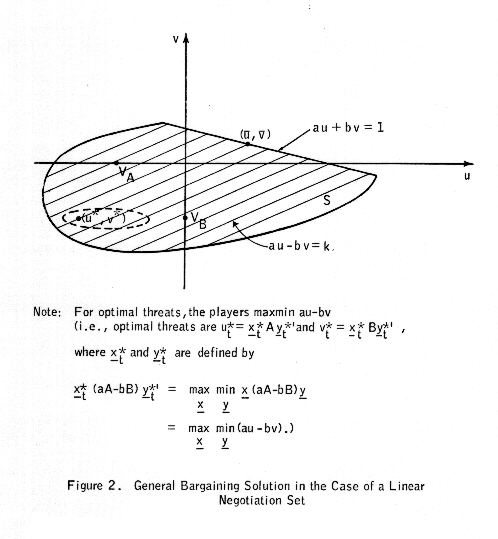
If the Pareto-optimal boundary of S is linear (au + bv = 1), then the strategies corresponding to the optimal threats are the maxmin solutions to the (zero-sum) matrix game
aA - bB .
This is easy to see. Subject to the constraint au + bv = 1, the values of u and v that maximize (u - u*) (v - v*) are
ub = (1/a + [u* - (b/a)v*])/2
and
vb = (a/b) (1/a - [u* - (b/a)v*)/2 .
Now u* = xAy' and v* = xBy' are the "status-quo" payoffs, or "threat" payoffs, to the respective players if they choose threat strategies x and y. Hence, in terms of x and y, we have
ub = (1/a + [x(A - (b/a)B)y'])/2
vb = (a/b) (1/a - [x(A - (b/a)B)y'])/2 .
Clearly, player 1 wishes to maximize
x(A - (b/a)B)y'
while player 2 wishes to minimize the same quantity. Hence the optimal threat strategies x and y are the minmax values xt and yt to the (zero-sum) matrix game A - (b/a)B, or, equivalently, to the matrix game aA - bB.
The situation is depicted in Figure 2. We define VA and VB to be the values of the two players' zero-sum games:
VA = max(x) min(y) xAy'
VB = max(y) min(x) xBy' .
We define
ut* = xtAyt'
and
vt* = xtByt'
where xt and yt are defined by
xt (aA -bB) yt' = max(x) min(y) x (aA - bB) y' .
For the graph, we have assumed that VA = VB, and that a is sufficiently smaller than b so that aA - bB is approximately equal to -bB. Hence vt* is approximately equal to VB, but ut* could vary considerably from VB. An interpretation of this situation is as follows. Since, relative to the value VB of his "threat" game B, player 2 has less to gain or lose through negotiations than player 1, he concentrates on holding player 1 to his minimum gain, rather than paying much attention to his own gain or loss. From the graph, we can see that this attitude is reasonable, since it is clear that fluctuations in the threat payoff ut* have much less effect on player 1's negotiated payoff ub than comparable fluctuations in vt* have on vb.
B. Hyperbolic Negotiation Set
1. Rectangular Hyperbola
If the Pareto-optimal boundary of S is nonlinear, then finding the optimal threats is not as straightforward as above. We shall investigate a situation which seems analogous to reality; namely, one in which the losses if the threats (war) are carried out are far greater than the gains from negotiation.
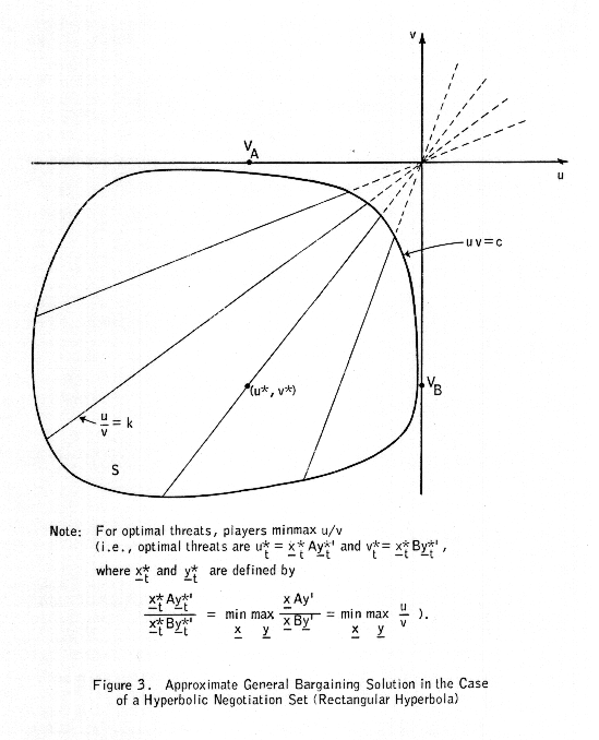
We assume that the negotiation set (Pareto-optimal boundary of S) can be approximated by the equation uv = c. Then we want to find values for u and v that maximize (u - u*)(v - v*) subject to uv = c. These values are
ub = -(cu*/v*)1/2
vb = -(cv*/u*)1/2 .
As before, u* = xAy' and v* = xBy' are the threat payoffs to players 1 and 2 if they choose threat strategies x and y, respectively. Clearly, player 1 wishes to minimize
u*/v* = xAy'/xBy'
while player 2 wishes to maximize this quantity. (This curious situation, in which player 1 wishes to minimize the ratio of his gains to those of player 2, occurs because all payoffs are negative. Were the negotiation set in the positive quadrant, there would be a more natural determinant of the optimal threat strategy.) Hence the optimal threat strategies for the players are the strategies xt and yt corresponding to
min(x) max(y) xAy'/xBy' .
Schroeder (Reference 2) suggests an iterative procedure for solving this ratio game. He notes that, if c denotes the value of the game, then the zero-sum game A - cB will have value zero; furthermore, optimal strategies for the zero-sum game A - cB are optimal for the ratio game. He suggests an iterative procedure for determining c (and hence optimal strategies xt and yt for the ratio game).
As an alternative to the iterative solution, the following approximate solution is suggested. Maximizing u*/v* is equivalent to maximizing ℓn u*/v* (where ℓn denotes the natural logarithm function). Let us denote the zero-sum solutions to the games A and B by (xA,yA) and (xB,yB), respectively. Then for xAy' close (in a percentage sense) to VA = xAAyA' and xBy' close to VB = xBByB' we can write
ℓn u* = ℓn xAy'
= ℓn (xAAyA' + xAy' - xAAyA')
= ℓn (VA + xAy' - VA)
approximately = ℓn VA + (1/VA)(xAy' - VA)
= ℓn VA + (1/VA)(xAy') - 1
and similarly,
ℓn v* approximately = ℓn VB + (1/VB)(xBy') - 1
so that
ℓn (u*/v*) approximately = ℓn (VA/VB) + (1/VA)xAy' - (1/VB)(xBy') ,
and hence, it seems reasonable to approximate
min(x) max(y) ℓn (u*/v*) approximately = min(x) max(y) (ℓn (VA/VB)
+ (1/VA)xAy' - (1/VB)xBy')
or
min(x) max(y) ℓn (u*/v*) approximately = ℓn (VA/VB)
+ min(x) max(y) x((1/VA)A - (1/VB)B)y' .
Hence near-optimal threat strategies xta and yta are those strategies corresponding to
min(x) max(y) x((1/VA)A - (1/VB)B)y' ,
i.e., to the solution of the (zero-sum) matrix game (1/VA)A - (1/VB)B. Hence we see that c is approximately equal to VA/VB, provided that the losses from combat are very large compared to the losses associated with negotiation.
The situation is described in Figure 3. As usual, VA and VB are the values of the zero-sum games A and B. We define
uta* = xtaAyta'
and
vta* = xtaByta'
where xta and yta are defined by
xta ((1/VA)A - (1/VB)B) yta' = min(x) max(y) x ((1/VA)A - (1/VB)B) y' .
If we assume that VA = VB, then xta and yta are the zero-sum solutions to the matrix game A - B.
The preceding approximate solution is noted
simply in passing. The really significant result of this section is that there
does exist a constant c such that the optimal threat strategies are solutions
of the zero-sum game A - cB. As noted earlier, the constant c is the solution
of the ratio game A/B and it therefore has the property that the zero-sum game
A - cB has value zero.
It is interesting to compare the threat strategies of the general-sum game in the case of a linear negotiation set to the approximate threat strategies in the case of a hyperbolic negotiation set. The zero-sum games that determine the threat strategies in these two cases are
aA - bB
and
(1/VA)A - (1/VB)B ,
or
(a/b)1/2 A - (b/a)1/2 B
and
(VB/VA)1/2 - (VA/VB)1/2 B ,
respectively.
It is noted that the derivations of this section are dependent upon the assumption that the center of the hyperbola defining the negotiation set is located at the origin, and that all payoffs are negative. If this assumption is removed, then c is such that the matrix game A - cB has some specified value different from zero, and c will no longer be approximately equal to VA/VB.
2. Nonrectangular Hyperbola
In reality, it would appear that there is a correlation between the losses to one player and losses to the other. That is, the feasible set S would tend to be "close" to the line u = cv. We shall now investigate this case.
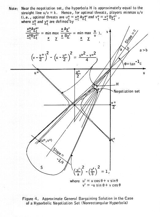
The situation is most easily described in terms of Figure 4. The problem is to find u = ub and v = vb that maximize
(u - u*)(v - v*)
subject to (u,v) being on the negotiation set of the boundary
((u cos θ + v sin θ)/a)2 - ((-u sin θ + v cos θ)/b)2 = 1 (1)
of S. The values ub and vb that maximize (u - u*)(v - v*) subject to (1) can be shown to be the solutions to the equations (1) and
(v - v*/2)2 - (u - u*/2)2 = (v*2 - u*2)/2 . (2)
In general, the solutions ub and vb
will lie on the boundary of S, but not in the negotiation set. This fact,
together with the fact that the above system of equations is difficult to
solve, makes it difficult to see what the optimal threat payoffs ut*
and vt* are. We hence look for an approximate solution. Note that,
since S is "long and narrow" and the threat payoffs are far from the
negotiation set, the two players will try to move u* and v* in opposite
directions along the line
u = -(1/c)v + k .
Hence player 1 is trying to minimize
u - cv
while player 2 is trying to maximize this same quantity. But
u - cv = x (A - cB) y' ,
and so approximate optimal threat strategies are the solutions xta and yta to the zero-sum (matrix) game
A - cB .
In order for S to be long and narrow, and lie along a line of slope c, the matrix A must be approximately equal to cB, in which case it is likely that VA = cVB, or c approximately = VA/VB. Hence the approximate optimal threat strategies are probably close to the solution to the game
A - (VA/VB)B
or the game
(1/VA)A - (1/VB)B ,
the same result as in the case of the rectangular hyperbolic negotiation set.
The following alternative method of reasoning reaches the same conclusion. The hyperbola defined by (2) asymptotically approaches the lines
u/v = u*/v* = k
say, and
u/(v - v*) = - (u*/v*) = -k .
(In fact, if u* = v*, the hyperbola degenerates into two crossed lines.) Only the first line is of interest, since it will be the line that intersects (or comes closest to) the negotiation set. Now player 1 wants the hyperbola defined by (2) to intersect the negotiation set as far to the right as possible. By the preceding observation, this is approximately the same as wanting the line u/v = k to intersect as far to the right as possible. Hence, since u and v are both negative, player 1 wishes (approximately) to minimize the ratio u/v = k, while player 2 wishes to maximize the same quantity. Hence approximately optimal threat strategies are the solutions to
min(x) max(y) u/v = min(x) max(y) (xAy')/(xBy') . (4)
Hence, from the results in the case of a rectangular hyperbolic negotiation set, approximately optimal threat strategies correspond to the solution of the zero-sum game A - cB, where c is the value of the ratio game A/B and hence has the property that the zero-sum game A - cB has value zero. As in the case of the rectangular hyperbolic negotiation set, approximately optimal threat strategies are those strategies xta and yta corresponding to
min(x) max(y) x ((1/VA)A - (1/VB)B) y' ,
i.e., to optimal solutions of the matrix game
(1/VA)A - (1/VB)B .
As before, the derivations of this section assume that the center of the hyperbola defining the negotiation set is located at the origin, and that all payoffs are negative.
3. The General Situation
Approximate Solution
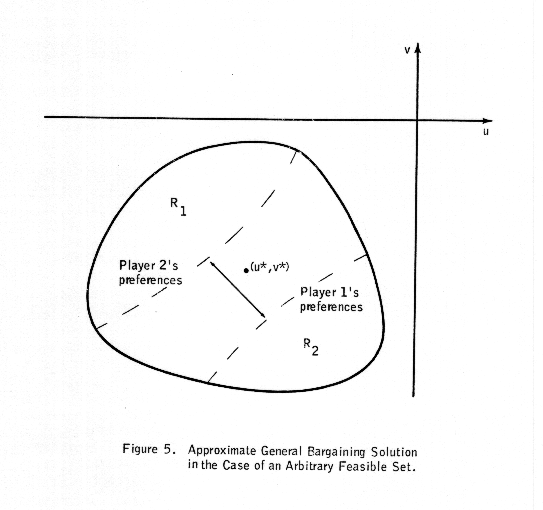
We shall now extend the results of the preceding section to the situation in which the negotiation set has neither a hyperbolic negotiation set nor a "long, narrow" shape. As illustrated in Figure 5, there are certain regions of the feasible set in which it is unreasonable to expect expected payoffs (such as the threat payoffs) to occur. For example, in order for the expected payoffs (u*,v*) to occur in region R1, player 1 would have to act in such a way that he tends to both minimize his own gains and those of his opponent. Similarly, in order for the expected payoffs to occur in region R2, player 2 would have to act in a similar fashion. Neither of these situations would correspond to those of "rational" strategies, regardless of the form of the negotiation set. Hence, "reasonable" pairs (u*,v*) tend to lie in a much narrower region than the entire feasible set. As usual, player 1 is attempting to push (u*,v*) toward R2, while player 2 is attempting to push (u*,v*) toward R1. Since the "reasonable" region is likely to be narrow, such efforts by the two players will correspond to their attempting to push (u*,v*) in opposite directions along lines approximately perpendicular to the narrow region. If the "reasonable" region is fairly straight, then these perpendicular lines are all of about the same slope, and hence the actions of the players correspond to playing a particular zero-sum game. The "reasonable" region would be fairly straight if the players' anticipated losses from war tended to be linearly proportional. Hence, to the extend that this last condition (proportional losses) holds, it is not difficult to determine (approximately) the zero-sum game to which the optimal strategies correspond.
To be perfectly explicit regarding the result
that we have derived, let us denote the "slope" of the
"reasonable" region by c. Then, the two players are in effect trying
to move the threat payoffs ut* and vt* in opposite
directions along a line
u = -(1/c)v + k .
Hence, as we observed in the preceding section, player 1 is trying to minimize
u - cv
while player 2 is trying to maximize this same quantity. But
u - cv = x (A -cB)) y' ,
and so the optimal threat strategies are the optimal solutions xt and yt to the zero-sum (matrix) game A - cB.
If the line through the optimal threat point and the corresponding bargaining solution passes near the origin, we can reason as before that
c approximately = VA/VB .
Exact Solution
We shall close this section with the observation that, even though the optimal threat strategies are in general not the optimal solutions of a zero-sum game involving a known linear combination of the matrices A and B, there does exist a zero-sum game whose optimal solutions are the optimal threat strategies. The usefulness of this result is conditioned by the fact that the matrix of this particular zero-sum game may depend on the optimal solution to the general-sum game. We shall first present a heuristic proof of the result, and then a precise derivation.
Let us refer to Figure 6. We denote the optimal threat payoffs by (ut*,vt*), and the corresponding bargaining solution by (ub,vb). Let us denote the slope of the line joining these two points by c*; i.e.,
c* = (ub - ut*)/(vb - vt*) .
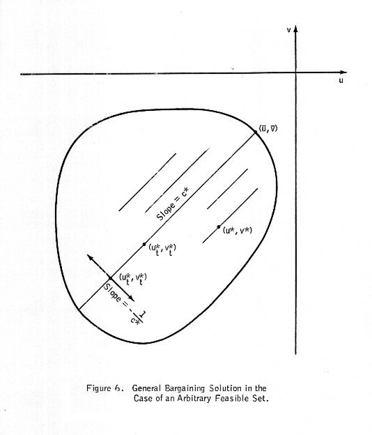
Let the equation of this line be u - c*v = k*.
At the optimal threat point (ut*,vt*) the two players are
attempting to move ut* and vt* in opposite directions
along the line of slope -1/c* through the point (ut*,vt*),
i.e., along the line
u + (1/c*)v = k' .
Consider the family of lines
u - c*v =k
parallel to the line
u - c*v = k*
joining the optimal threat point and the corresponding bargaining solution. Since (ut*,vt*) is the threat point optimal for both players, then by the reasoning used earlier in this section, we must have
k* = min(x) max(y) k
which holds if
ut* - c*vt* = min(x) max(y) (u* - c*v*)
or
xtAyt' - c*xtByt' = min(x) max(y) (xAy' - c*xBy)
or
xt (A - c*B) yt' = min(x) max(y) x (A - c*B) y' .
Thus the optimal strategies (xt,yt) for the matrix game
A - c*B
are optimal threat strategies for the nonzero-sum game. Thus we have shown that there does exist a zero-sum game whose optimal strategies are optimal threat strategies. Unfortunately, this zero-sum game (A - c*B) depends on c*, which is known only after we in fact have the solution to the problem we are attempting to solve. Note that the value of the game A - c*B must be k*, which is also unknown. As Schroeder (Reference 2) has noted (for the case k* = 0), if we know the value of k*, then we can determine c* (and hence the optimal strategies (xt,yt)) iteratively, by choosing a trial value ca* for c*, and adjusting the trial value if the value of the game A - ca*B differs "too" much from k*. Note that if the negotiation set is "near" (relative to the rest of the feasible set) the origin, then k* is "close" to zero.
We now present a rigorous derivation of the preceding result. We assume that u < 0 and v < 0 for all (u,v) in the feasible set; that the negotiation set is defined by a continuously differentiable curve f(u,v) = 0; that the family of straight lines intersecting f(u,v) = 0 and having slope negative to that of f at the point of intersection is defined by a continuously differentiable function g(u,v) = k, where the various lines are defined by varying the parameter k. Let the straight line corresponding to g(u,v) = k be u - c(k)v = h(c). Let (u*,v*) denote the optimal threat point. Now as we vary u, the parameter c of the function g also varies, but, by the nature of the negotiation set, we must have Δc/ Δu ≥ 0. Similarly, we have Δc/ Δv ≤ 0. Now, by optimality, if
g(u*,v*) = k*
then
g(u* + Δu,v*) ≤ k*
and
g(u*,v* + Δv) ≥ k* .
That is,
(u* + Δu) - (c* + Δc/ Δu)v* ≤ k*
or
(u* + Δu) - c*v* ≤ k* + v*( Δc/ Δu) ≤ k*
since v* < 0 and Δc/ Δu ≥ 0.
Also,
u* - (c* + Δc/ Δv)(v* + Δv) ≥ k*
or
u* - c*(v* + Δv) ≥ k* + v*( Δc/ Δv) ≥ k*
since v* < 0, and Δc/ Δv ≤ 0. Hence, since u* - c*v* = k*, the optimal threat strategies u* and v* are the optimal solutions to the zero-sum game A - c*B. Furthermore, this game has value k*.
Note that the principal assumption made above is that all payoffs are negative. Unless some assumption is made that will restrict the value of k*, however, the result does not appear to be very useful from a computational viewpoint. If we know the value of k*, then we can iteratively determine the value of c*, and (simultaneously) the optimal threat strategies. if the negotiation set is "close" (relative to the remainder of the feasible set) to the origin, then k* is approximately equal to zero. As we noted earlier, if the expected losses for the two players tend to be proportional, then c* is the proportionality constant (and k* is the u-intercept of the line of proportionality).
V. A Real-World Implication
In general, it appears that many negotiation and conflict situations in the real world would have the essential characteristics of the situations of the previous section: essentially, expected losses that are large compared to the payoff for negotiation. Hence it is felt that, in optimization problems involving war between two parties, a reasonable payoff function for both parties to examine in conducting the war is the matrix A - cB, where A and B are the respective parties' payoff matrices and c is chosen so that the value of the matrix game A - cB is zero. (Note that here we are assuming that the two players' payoff functions are translated so that the feasible set is in the lower left quadrant, close to the origin.) Furthermore, c is approximately equal to VA/VB, where VA and VB denote the values of the matrix games A and B.
The above result appears to be a useful one, since it provides the military analyst with a zero-sum game representation of war that is generally consistent with the general-sum formulation of negotiation and conflict. The result hence offers the advantage of retaining computational simplicity (since it deals with zero-sum games) while appearing to be a more adequate representation of the real world.
A drawback associated with implementation of the preceding result is that the matrices A and B must specify payoffs resulting from all possible actions: those resulting from negotiations and those resulting from conflict. It is noted, however, that the preceding result is not heavily dependent on the slope of the negotiation set but only on its general location. We shall now heuristically derive a useful implication of this situation, for the case in which the only payoffs we know are those corresponding to conflict (and we assume that the negotiation set is "far" from the "conflict set"). We shall here use the approximation that c is approximately equal to VA/VB.
We suppose, then, that it is possible to define payoffs corresponding to military actions that are likely to result from failure of negotiations. Thus we assume knowledge of submatrices As and Bs of A and B; the matrices As and Bs define the payoffs corresponding to feasible military actions. It seems reasonable to assume that the values of the zero-sum games As and Bs would be close to the values of the zero-sum games A and B, since if player 1's losses are equivalent to player 2's gains, it is obviously to player 2's advantage in the zero-sum game A to declare war, and similarly to player 1's advantage in the zero sum game B to declare war. (The underlying assumption here is that waging war is costly, whereas negotiation is not.) Thus we assume that
VA approximately = VAs
and that
VB approximately = VBs .
For the same reason, it appears reasonable to assume that in the zero-sum game
(1/VA)A - (1/VB)B ,
the strategies of primary interest correspond to military actions. Hence the optimal strategies for the zero-sum game
(1/VA)A - (1/VB)B
are likely to be similar to those for the zero-sum game
(1/VA)As - (1/VB)Bs .
But since VA approximately = VAs and VB approximately = VBs, the game is approximately the same as the game
(1/VAs)As - (1/VBs)Bs .
Hence, it appears that military analysts should examine the zero-sum game
(1/VAs)As - (1/VBs)Bs
in their analyses. This result appears to be a useful one in that it does not place on the military analysts the burden of identifying the negotiation set.
References
1. Owen. G., Game Theory, W. B. Saunders Co., Philadelphia, 1968.
2. Schroeder, R. G., "Linear Programming Solutions to Ratio Games," Operations Research, April, 1970, Vol. 18, No. 2, pp. 300-305.
FndID(29)
FndTitle(Conflict, Negotiation, and General-Sum Game Theory)
FndDescription(This paper examines the problem of determining a computationally tractable general-sum game-theoretic solution to war, taking into account the effect of the threat of war on negotiations.)
FndKeywords(nonzerol sum game; general sum game; positive sum game; bimatrix game; nash's bargaining solution; pareto optimal)